1 Inroduction
One of the key ideas behind ggplot2 is that it allows you to easily iterate, building up a complex plot a layer at a time, which is composed of five parts:
- Data.
- Aesthetic mappings.
- A statistical transformation (stat).
- A geometric object (geom).
- A position adjustment.
2 Build a plot layer by layer
It’s important to realize that there’s nothing to see until we add a layer, which is created by the layer() function. geom_point is a shortcut of this function.
p <- ggplot(mpg, aes(displ, hwy))
p |
# the same as geom_point
p + layer(mapping = NULL,
          data = NULL,
          geom = "point",
          stat = "identity",
          position = "identity")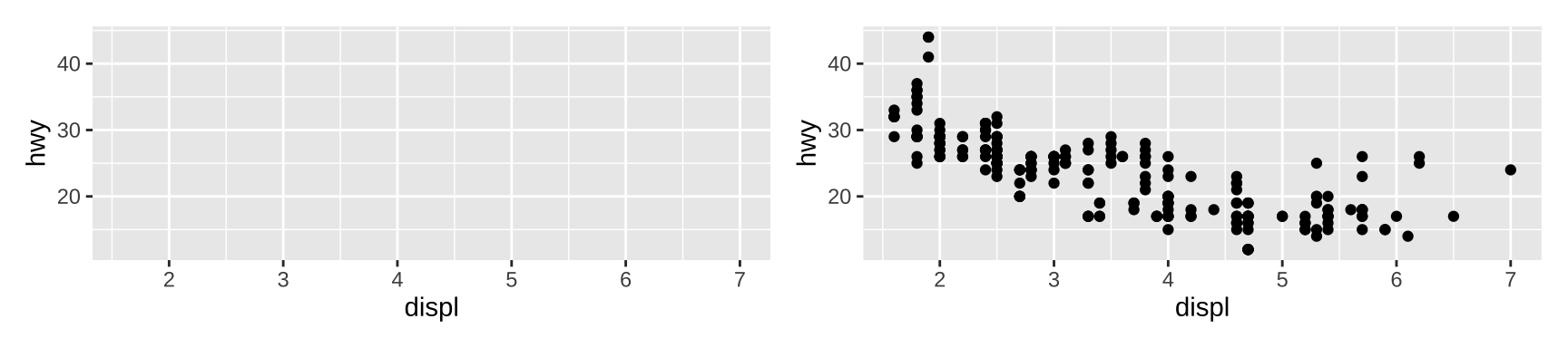
2.1 Data
Never refer to a variable with $ in aes() (e.g., diamonds$carat). This breaks containment, so that the plot no longer contains everything it needs, and causes problems if ggplot2 changes the order of the rows, as it does when faceting.
library(dplyr)
class <- mpg %>%
  group_by(class) %>%
  summarise(n = n(), hwy = mean(hwy))
# my answer
ggplot(mpg,aes(class,hwy))+
  geom_jitter(color="black")+
  geom_point(aes(class,hwy),class,color="red",size=4)+
  annotate("text",x=1:length(unique(mpg$class)),y=10,
           label=paste0("n = ",class$n))|
# the answer provided by the author
ggplot(mpg, aes(class, hwy)) +
  geom_jitter(width = 0.25) +
  geom_point(data = class, colour = "red", size = 4) +
  geom_text(aes(y = 10, label = paste0("n = ", n)),
            class, size = 3)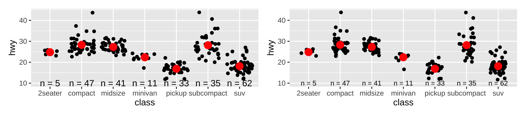
2.2 Aesthetic mappings
Aesthetic mappings can be supplied in the initial ggplot() call, in individual layers, or in some combination of both. The way you specify aesthetics doesn’t make any difference if there’s only one layer, but the distinction is important when you start adding additional layers.
ggplot(mpg, aes(displ, hwy, colour = class)) +
  geom_point() +
  geom_smooth(method = "lm", se = FALSE) +
  theme(legend.position = "none")|

ggplot(mpg, aes(displ, hwy)) +
  geom_point(aes(colour = class)) +
  geom_smooth(method = "lm", se = FALSE) +
  theme(legend.position = "none")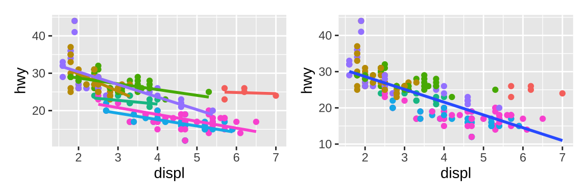
If you want appearance to be governed by a variable, put the specification inside aes(); if you want override the default size or color, put the value outside of aes(). Another way to override the default scale is using scale_colour_identity(). It’s sometimes useful to map aesthetics to constants.
ggplot(mpg, aes(cty, hwy)) +
  geom_point(aes(color = "blue")) +
  scale_color_identity()|
ggplot(mpg, aes(displ, hwy)) +
  geom_point() +
  geom_smooth(aes(color = "loess"), method = "loess", se = FALSE) +
  geom_smooth(aes(color = "lm"), method = "lm", se = FALSE) +
  labs(color = "Method")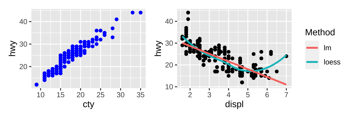
2.3 Geoms
Geometric objects, or geoms for short, perform the actual rendering of the layer. Here are some geoms I’m not familiar with:
- Graphical primitives:
geom_blank(): display nothing. Most useful for adjusting axes limits using data.geom_ribbon(): ribbons, a path with vertical thickness.geom_segment(): a line segment, specified by start and end position.geom_polygon(): filled polygons.geom_text(): text.
- One variable:
- Discrete:
geom_histogram(): bin and count continuous variable, display with bars.geom_density(): smoothed density estimate.geom_dotplot(): stack individual points into a dot plot.geom_freqpoly(): bin and count continuous variable, display with lines.
- Discrete:
- Two variables:
- Both continuous:
geom_quantile(): smoothed quantile regression.geom_rug(): marginal rug plots.geom_text(): text labels.
- Show distribution:
geom_bin2d(): bin into rectangles and count.geom_density2d(): smoothed 2d density estimate.geom_hex(): bin into hexagons and count.
- At least one discrete:
geom_count(): count number of point at distinct locations
- One continuous, one discrete:
geom_bar(stat = "identity"): a bar chart of precomputed summaries.
- One time, one continuous
geom_step(): step plot.
- Display uncertainty:
geom_crossbar(): vertical bar with center.geom_map(): fast version ofgeom_polygon()for map data.
- Both continuous:
- Three variables:
geom_contour(): contours.geom_raster(): fast version ofgeom_tile()for equal sized tiles.
Each geom has a set of aesthetics that it understands, some of which must be provided. For example, a bar requires height (ymax), and understands width, border color and fill color.
Some geoms differ primarily in the way that they are parameterised. For example, you can draw a square in three ways:
geom_tile(): the location (xandy) and dimensions (widthandheight).geom_rect(): top (ymax), bottom (ymin), left (xmin) and right (xmax) positions.geom_polygon(): a four row data frame with thexandypositions of each corner.
2.4 Stats
A statistical transformation, or stat, transforms the data, typically by summarising it. You’ve already used many of ggplot2’s stats because they’re used behind the scenes to generate many important geoms:
stat_bin():geom_bar(),geom_freqpoly(),geom_histogram()stat_bin2d():geom_bin2d()stat_bindot():geom_dotplot()stat_binhex():geom_hex()stat_boxplot():geom_boxplot()stat_contour():geom_contour()stat_quantile():geom_quantile()stat_smooth():geom_smooth()stat_sum():geom_count()
You’ll rarely call these functions directly, but they are useful to know about because their documentation often provides more detail about the corresponding statistical transformation.
Other stats can’t be created with a geom_ function:
stat_ecdf(): compute a empirical cumulative distribution plot.stat_function(): compute y values from a function of x values.stat_summary(): summarise y values at distinct x values.stat_summary2d(),stat_summary_hex(): summarise binned values.stat_qq(): perform calculations for a quantile-quantile plot.stat_spoke(): convert angle and radius to position.stat_unique(): remove duplicated rows.
There are two ways to use these functions. You can either add a stat_() function and override the default geom, or add a geom_() function and override the default stat:
ggplot(mpg, aes(trans, cty)) +
  geom_point() +
  stat_summary(geom = "point", fun = "mean",
               colour = "red", size = 4)|
ggplot(mpg, aes(trans, cty)) +
  geom_point() +
  geom_point(stat = "summary", fun = "mean",
             colour = "red", size = 4)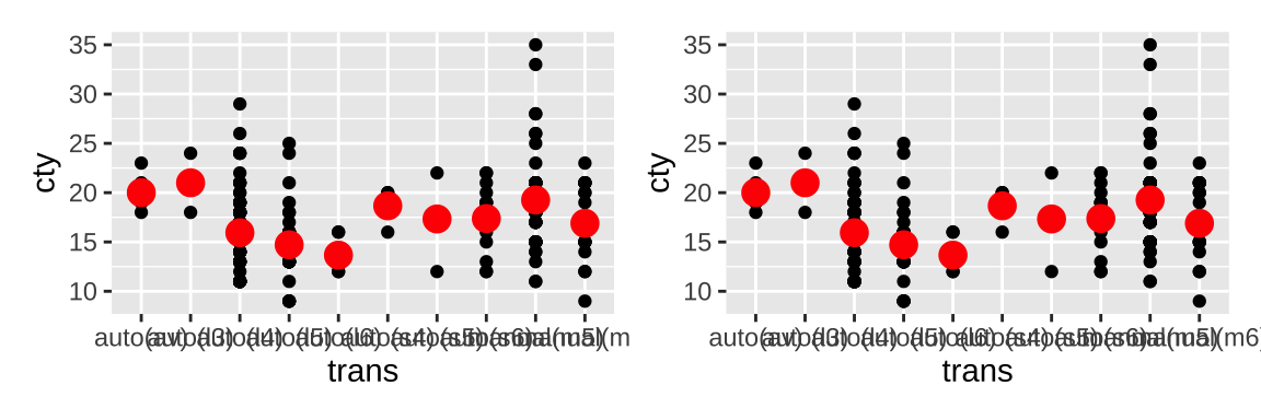
Internally, a stat takes a data frame as input and returns a data frame as output, and so a stat can add new variables to the original dataset. To refer to a generated variable like density, after_stat() must wrap the name.
ggplot(diamonds, aes(price, colour = cut)) +
  geom_freqpoly(binwidth = 500) +
  theme(legend.position = "none") |

ggplot(diamonds, aes(price, colour = cut)) +
  geom_freqpoly(aes(y = after_stat(density)), binwidth = 500) +
  theme(legend.position = "none")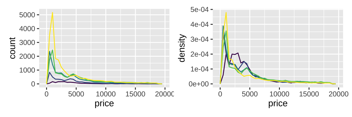
2.5 Position adjustments
Position adjustments apply minor tweaks to the position of elements within a layer. Three adjustments apply primarily to bars:
position_stack(): stack overlapping bars (or areas) on top of each other.position_fill(): stack overlapping bars, scaling so the top is always at 1.position_dodge(): place overlapping bars (or boxplots) side-by-side.position_identity(): do nothing.
dplot <- ggplot(diamonds, aes(color, fill = cut)) +
  xlab(NULL) + ylab(NULL) + theme(legend.position = "none")
# position stack is the default for bars, so `geom_bar()`
# is equivalent to `geom_bar(position = "stack")`.
dplot + geom_bar()|
dplot + geom_bar(position = "fill")|
dplot + geom_bar(position = "dodge")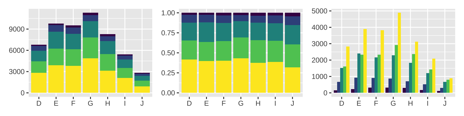
There are three position adjustments that are primarily useful for points:
position_nudge(): move points by a fixed offset.position_jitter(): add a little random noise to every position.position_jitterdodge(): dodge points within groups, then add a little random noise.
ggplot(mpg, aes(displ, hwy)) +
  geom_point(position = "jitter")|
ggplot(mpg, aes(displ, hwy)) +
  geom_point(position = position_jitter(width = 0.05, height = 0.5))|
# geom_jitter() is a shortcut
ggplot(mpg, aes(displ, hwy)) +
  geom_jitter(width = 0.2, height = 0.8)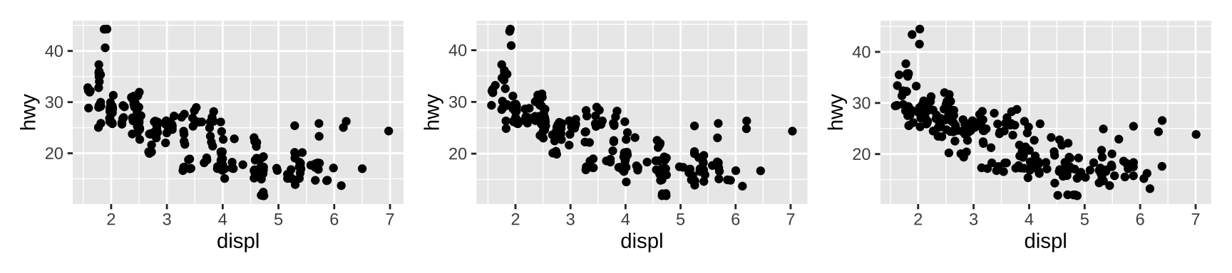
3 Scales and guides
The use of + to “add” scales to a plot is a little misleading because if you supply two scales for the same aesthetic, the last scale takes precedence.
All scale functions in ggplot2 belong to one of three fundamental types:
- continuous scales
- discrete scales
- binned scales
Each fundamental type is handled by one of three scale constructor functions;
continuous_scale(),discrete_scale()andbinned_scale().
3.1 Scale transformation
The linearly mapped scale on the left makes it easy to see the peaks of the distribution, whereas the transformed representation on the right makes it easier to see the regions of non-negligible density around those peaks:
base <- ggplot(faithfuld, aes(waiting, eruptions)) +
  geom_raster(aes(fill = density)) +
  scale_x_continuous(NULL, NULL, expand = c(0, 0)) +
  scale_y_continuous(NULL, NULL, expand = c(0, 0))

base|
base + scale_fill_continuous(trans = "sqrt")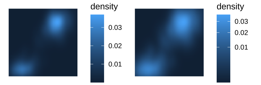
3.2 Scale guides
In ggplot2, legend and axes are known collectively as guides, which allow you to read observations from the plot or map them back to their original values.
| Argument name | Axis | Legend |
|---|---|---|
name |
Label | Title |
breaks |
Ticks & grid line | Key |
labels |
Tick label | Key label |
3.3 Scale breaks
Where labs() provides a shorthand way to specify the name argument to one or more scales, the guides() function allows you to specify guide arguments to one or more scales. In the same way that labs(colour = "a colour scale name") specifies the name associated with the color scale, a command such as guides(colour = guide_coloursteps()) can be used to specify its associated guide:
base <- ggplot(mpg, aes(displ, hwy, colour = cyl)) + geom_point()

base |
base + scale_colour_continuous(guide = guide_coloursteps())|
base + guides(colour = guide_coloursteps())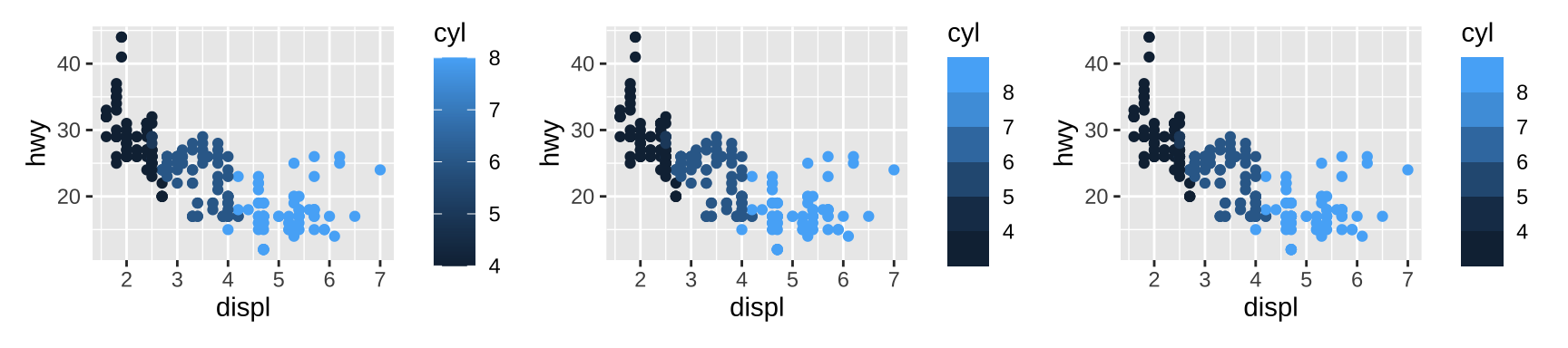
Scale guides are more complex than scale names: where the name argument (and labs() ) takes text as input, the guide argument (and guides()) require a guide object created by a guide function:
| Scale type | Default guide type |
|---|---|
| continuous scales for colour/fill aesthetics | colourbar |
| binned scales for colour/fill aesthetics | coloursteps |
| position scales (continuous, binned and discrete) | axis |
| discrete scales (except position scales) | legend |
| binned scales (except position/colour/fill scales) | bins |
3.4 Legend merging and splitting
By default, a layer will only appear if the corresponding aesthetic is mapped to a variable with aes(). You can override whether or not a layer appears in the legend with show.legend.
toy <- data.frame(
  const = 1,
  up = 1:4,
  txt = letters[1:4],
  big = (1:4)*1000,
  log = c(2, 5, 10, 2000)
)
ggplot(toy, aes(up, up)) +
  geom_point(size = 4, colour = "grey20") +
  geom_point(aes(colour = txt), size = 2) |
# show grey points in legend
ggplot(toy, aes(up, up)) +
  geom_point(size = 4, colour = "grey20", show.legend = TRUE) +
geom_point(aes(colour = txt), size = 2) 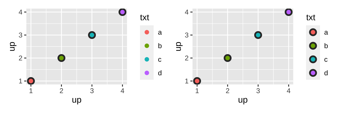
The ggnewscale::new_scale_colour() command acts as an instruction to ggplot2 to initialize a new color scale: scale and guide commands that appear above the new_scale_colour() command will be applied to the first color scale, and commands that appear below are applied to the second color scale.
base <- ggplot(mpg, aes(displ, hwy)) +
  geom_point(aes(colour = factor(year)), size = 5) +
  scale_colour_brewer("year", type = "qual", palette = 5)

base|
base +
  ggnewscale::new_scale_colour() +
  geom_point(aes(colour = cyl == 4), size = 1, fill = NA) +
  scale_colour_manual("4 cylinder", values = c("grey60", "black"))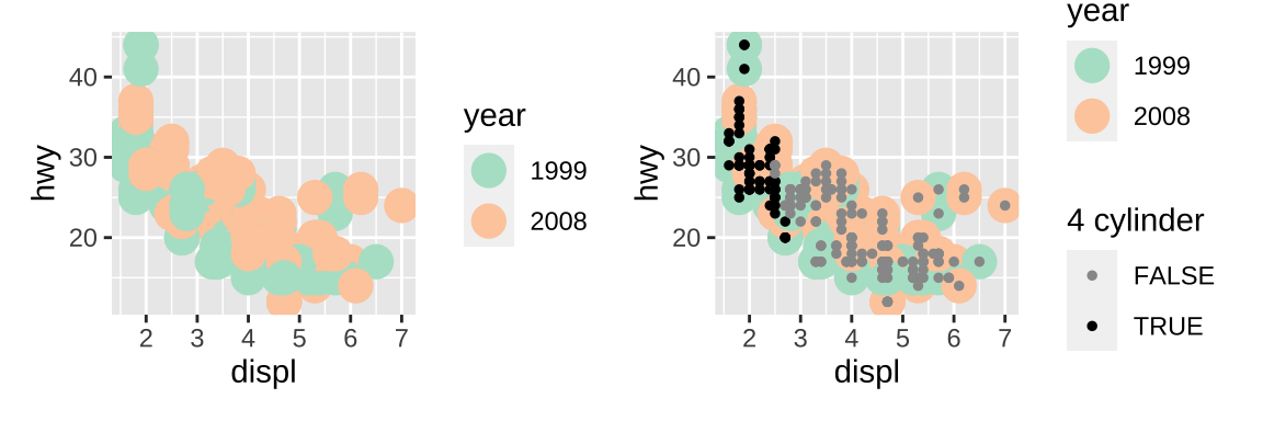
4 Coordinate systems
4.1 Linear coordinate systems
coord_cartesian(): the default Cartesian coordinate system, where the 2d position of an element is given by the combination of the x and y positions.
coord_flip(): Cartesian coordinate system with x and y axes flipped.coord_fixed(): Cartesian coordinate system with a fixed aspect ratio.
ggplot(mpg, aes(displ, cty)) +
  geom_point() +
  geom_smooth()|
# exchange x and y
ggplot(mpg, aes(cty, displ)) +
  geom_point() +
  geom_smooth()|
# flip coord
ggplot(mpg, aes(displ, cty)) +
  geom_point() +
  geom_smooth() +
  coord_flip()|
# set ratio and ylim
ggplot(mpg, aes(displ, cty)) +
  geom_point() +
  geom_smooth() +
  coord_fixed(ratio=1/2,ylim = c(10,30))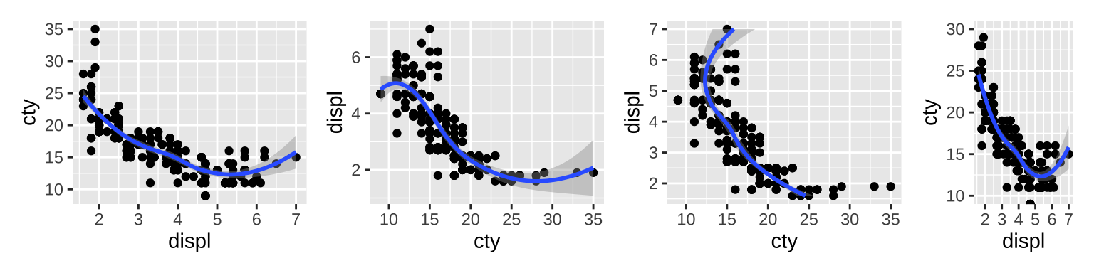
4.2 Non-linear coordinate systems
coord_map()/coord_quickmap()/coord_sf(): Map projections.coord_polar(): Polar coordinates.coord_trans(): Apply arbitrary transformations to x and y positions, after the data has been processed by the stat.
rect <- data.frame(x = 50, y = 50)
line <- data.frame(x = c(1, 200), y = c(100, 1))
base <- ggplot(mapping = aes(x, y)) +
  geom_tile(data = rect, aes(width = 50, height = 50)) +
  geom_line(data = line) +
  xlab(NULL) + ylab(NULL)
base|
base + coord_trans(y = "log10")|
# theta argument determines which position variable
# is mapped to angle (by default, x)
base + coord_polar()|
base + coord_polar("y")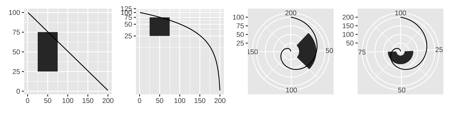
Maps are intrinsically displays of spherical data. Simply plotting raw longitudes and latitudes is misleading, so we must project the data. There are two ways to do this with ggplot2:
coord_quickmap(): quick and dirty approximation that sets the aspect ratio to ensure that 1m of latitude and 1m of longitude are the same distance in the middle of the plot.coord_map(): uses the mapproj package, to do a formal map projection. It takes the same arguments asmapproj::mapproject()for controlling the projection. It is much slower thancoord_quickmap()because it must munch (cut into pieces) the data and transform each piece.
# Polygons are very similar to paths (as drawn by geom_path())
# except that the start and end points are connected
# and the inside is colored by fill.
world <- map_data("world")
worldmap <- ggplot(world, aes(long, lat, group = group)) +
  geom_path() +
  scale_y_continuous(NULL, breaks = (-2:3) * 30, labels = NULL)+
  scale_x_continuous(NULL, breaks = (-4:4) * 45, labels = NULL)+
  theme(axis.ticks = element_blank())
# maximum longitude in world exceed 180,
# causing strange lines on the map.
# Setting xlim can fix it.
worldmap + coord_map(xlim=c(-180,180))|
# Some crazier projections
worldmap + coord_map("ortho",xlim=c(-180,180))|
worldmap + coord_quickmap()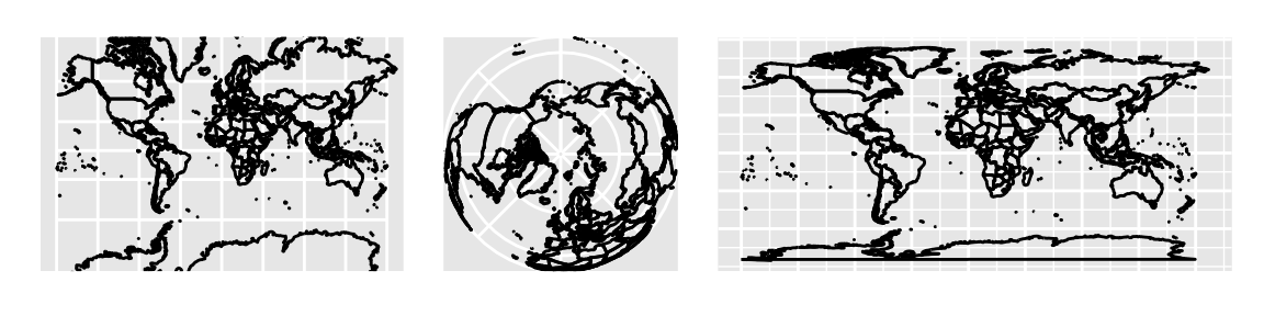
5 Faceting
There are three types of faceting:
- facet_null(): a single plot, the default.
- facet_wrap(): “wraps” a 1d ribbon of panels into 2d.
- facet_grid(): produces a 2d grid of panels defined by variables which form the rows and columns.
5.1 Facet wrap
facet_wrap() wraps a long ribbon of panels into 2d. as.table controls whether the facets are laid out like a table (TRUE), with highest values at the bottom-right, or a plot (FALSE), with the highest values at the top-right. dir controls the direction of wrap: horizontal or vertical.
mpg2 <- subset(mpg, cyl != 5 & drv %in% c("4", "f") & class != "2seater")

base <- ggplot(mpg2, aes(displ, hwy)) +
  geom_blank() +
  xlab(NULL) +
  ylab(NULL)

base + facet_wrap(~class, ncol = 3)|
base + facet_wrap(~class, ncol = 3, as.table = FALSE)|
base + facet_wrap(~class, ncol = 3, dir = "v")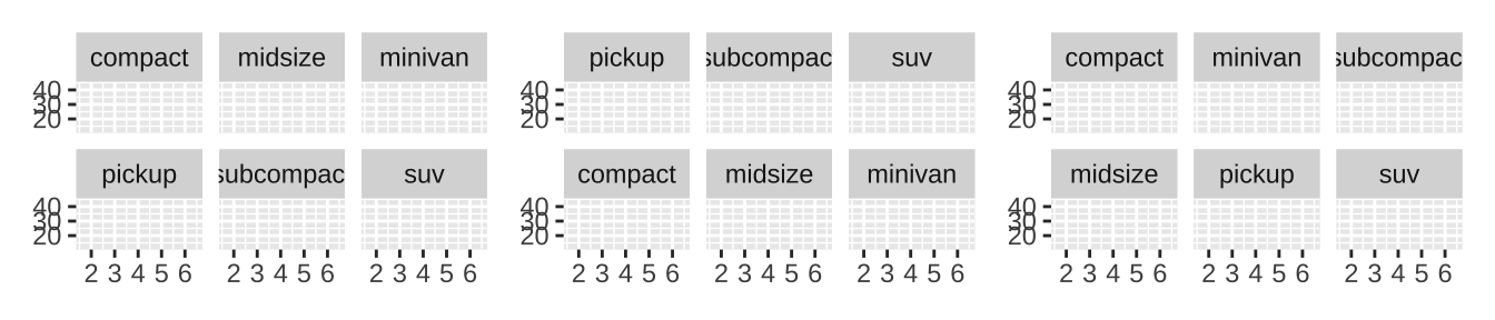
5.2 Facet grid
facet_grid() lays out plots in a 2d grid, as defined by a formula:
. ~ aspreads the values of a across the columns.b ~ .spreads the values of b down the rows.a ~ bspreads a across columns and b down rows.- You can use multiple variables in the rows or columns, by “adding” them together, e.g.
a + b ~ c + d.
base + facet_grid(drv ~ cyl)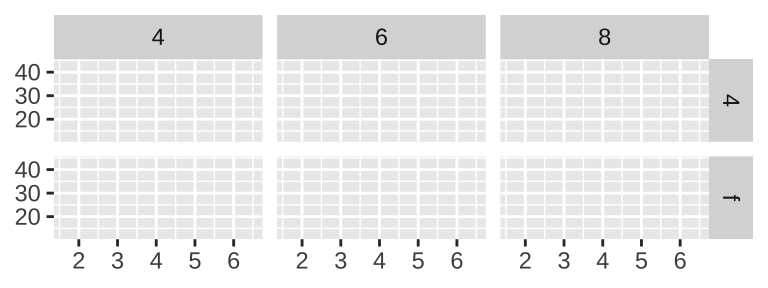
5.3 Controlling scales
For both facet_wrap() and facet_grid() you can control whether the position scales are the same in all panels (fixed) or allowed to vary between panels (free) with the scales parameter:
scales = "fixed": x and y scales are fixed across all panels.scales = "free_x": the x scale is free, and the y scale is fixed.scales = "free_y": the y scale is free, and the x scale is fixed.scales = "free": x and y scales vary across panels.
facet_grid() has an additional parameter called space, which takes the same values as scales. When space is “free”, each column (or row) will have width (or height) proportional to the range of the scale for that column (or row). This makes the scaling equal across the whole plot: 1 cm on each panel maps to the same range of data.
mpg2$model <- reorder(mpg2$model, mpg2$cty)
mpg2$manufacturer <- reorder(mpg2$manufacturer, -mpg2$cty)
ggplot(mpg2, aes(cty, model)) +
  geom_point() +
  facet_grid(manufacturer ~ ., scales = "free", space = "free") +
  theme(strip.text.y = element_text(angle = 0))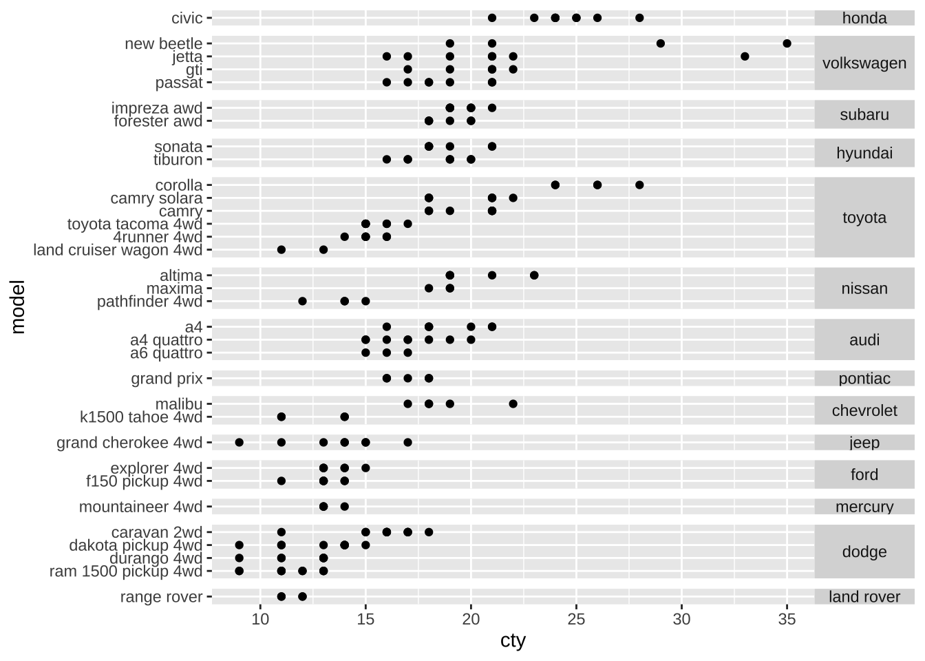
5.4 Missing faceting variables
When one of the dataset is missing a faceting variable, ggplot will display the map in every facet: missing faceting variables are treated like they have all values.
df1 <- data.frame(x = 1:3, y = 1:3, gender = c("f", "f", "m"))
df2 <- data.frame(x = 2, y = 2)

ggplot(df1, aes(x, y)) +
  geom_point(data = df2, colour = "red", size = 2) +
  geom_point() +
  facet_wrap(~gender)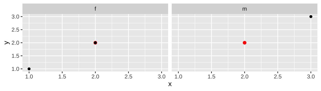
6 Themes
The theming system is composed of four main components:
- Theme elements specify the non-data elements that you can control. For example, the
plot.titleelement controls the appearance of the plot title;axis.ticks.x, the ticks on the x axis;legend.key.height, the height of the keys in the legend. - Each element is associated with an element function, which describes the visual properties of the element. For example,
element_text()sets the font size, color and face of text elements likeplot.title. - The
theme()function which allows you to override the default theme elements by calling element functions, liketheme(plot.title = element_text(colour = "red")). - Complete themes, like
theme_grey()set all of the theme elements to values designed to work together harmoniously.
6.1 Complete themes
ggplot2 comes with a number of built in themes:
theme_grey(): a theme with a light grey background and white gridlines.theme_bw(): a variation ontheme_grey()that uses a white background and thin grey grid lines.theme_linedraw(): A theme with only black lines of various widths on white backgrounds, reminiscent of a line drawing.theme_light(): similar totheme_linedraw()but with light grey lines and axes, to direct more attention towards the data.theme_dark(): the dark cousin oftheme_light(), with similar line sizes but a dark background. Useful to make thin colored lines pop out.theme_minimal(): A minimalistic theme with no background annotations.theme_classic(): A classic-looking theme, with x and y axis lines and no gridlines.theme_void(): A completely empty theme.
df <- data.frame(x = 1:3, y = 1:3)
base <- ggplot(df, aes(x, y)) + geom_point()
figure <- list()
figure[[1]] <- base + theme_grey() + ggtitle("theme_grey()")
figure[[2]] <- base + theme_bw() + ggtitle("theme_bw()")
figure[[3]] <- base + theme_linedraw() + ggtitle("theme_linedraw()")
figure[[4]] <- base + theme_light() + ggtitle("theme_light()")
figure[[5]] <- base + theme_dark() + ggtitle("theme_dark()")
figure[[6]] <- base + theme_minimal()  + ggtitle("theme_minimal()")
figure[[7]] <- base + theme_classic() + ggtitle("theme_classic()")
figure[[8]] <- base + theme_void() + ggtitle("theme_void()")
wrap_plots(figure,ncol = 4)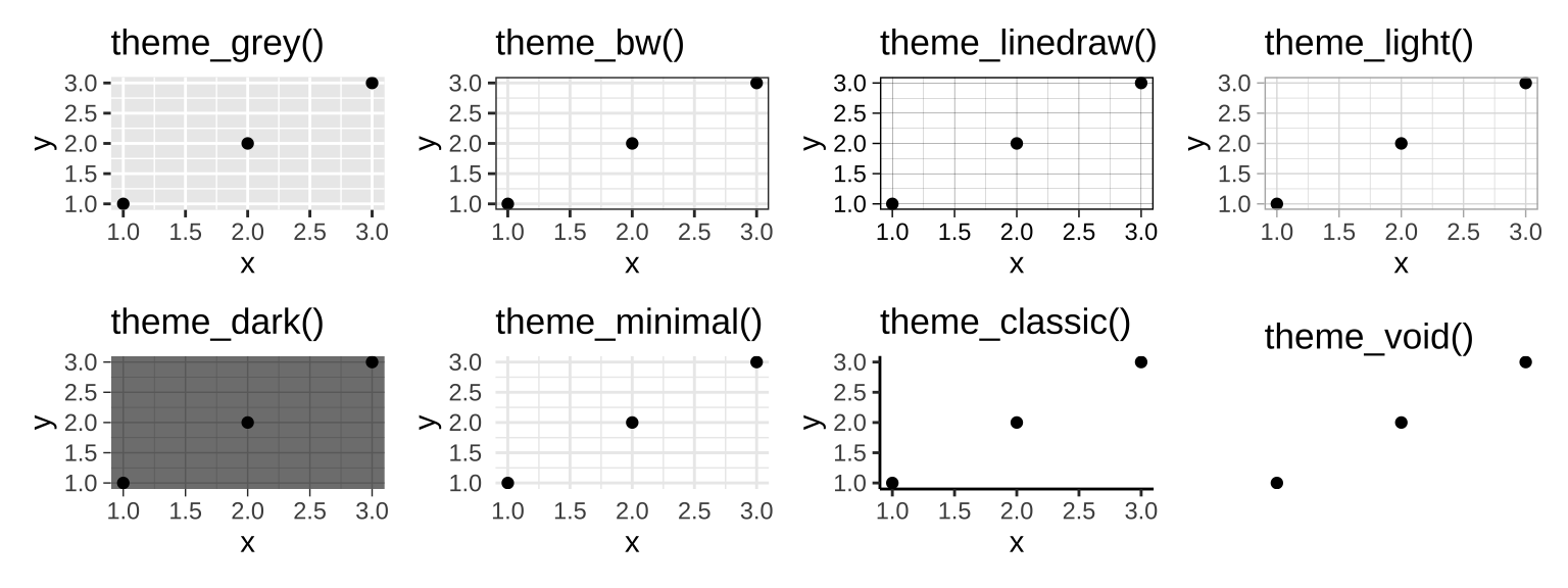
All themes have a base_size parameter which controls the base font size. As well as applying themes a plot at a time, you can change the default theme with theme_set(), such as theme_set(theme_bw()).
6.2 Modifying theme components
To modify an individual theme component you use code like plot + theme(element.name = element_function()).
Here are four basic types of built-in element functions: text, lines, rectangles, and blank.
element_text()draws labels and headings. You can control the fontfamily,face,colour,size(in points),hjust,vjust,angle(in degrees) andlineheight(as ratio offontcase). More details on the parameters can be found invignette("ggplot2-specs"). Margins around the text are controlled by themarginargument andmargin()function.element_line()draws lines parameterised bycolour,sizeandlinetypeelement_rect()draws rectangles, mostly used for backgrounds, parameterised byfillcolour and bordercolour,sizeandlinetype.element_blank()draws nothing. Use this if you don’t want anything drawn, and no space allocated for that element. A few other settings take grid units. Create them withunit(1, "cm")orunit(0.25, "in").
To modify theme elements for all future plots, use theme_update(). It returns the previous theme settings (theme_set also returns the old theme), so you can easily restore the original parameters.
old_theme <- theme_update(
  plot.background = element_rect(fill = "lightblue3", colour = NA),
  panel.background = element_rect(fill = "lightblue", colour = NA),
  axis.text = element_text(colour = "linen"),
  axis.title = element_text(colour = "linen")
)
# plot with new theme and set back to old theme
base + theme_set(old_theme)|
base # old theme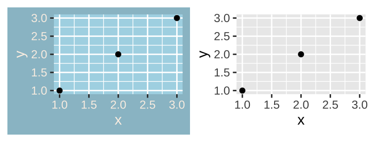
6.3 Theme elements
There are around 40 unique elements that control the appearance of the plot. They can be roughly grouped into five categories: plot, axis, legend, panel and facet.
6.3.1 Plot elements
| Element | Setter | Description |
|---|---|---|
| plot.background | element_rect() |
plot background |
| plot.title | element_text() |
plot title |
| plot.margin | margin() |
margins around plot |
To make the background transparent, set fill = NA.
6.3.2 Axis elements
| Element | Setter | Description |
|---|---|---|
| axis.line | element_line() |
line parallel to axis |
| axis.text | element_text() |
tick labels |
| axis.text.x | element_text() |
x-axis tick labels |
| axis.text.y | element_text() |
y-axis tick labels |
| axis.title | element_text() |
axis titles |
| axis.title.x | element_text() |
x-axis title |
| axis.title.y | element_text() |
y-axis title |
| axis.ticks | element_line() |
axis tick marks |
| axis.ticks.length | unit() |
length of tick marks |
Note that axis.line is hidden in default themes. axis.text (and axis.title) comes in three forms: axis.text, axis.text.x, and axis.text.y. Use the first form if you want to modify the properties of both axes at once. For example. setting axis.text.x = element_text(angle = -30, vjust = 1, hjust = 0) could adjust axis.text.x that avoid overlapping.
6.3.3 Legend elements
| Element | Setter | Description |
|---|---|---|
| legend.background | element_rect() |
legend background |
| legend.key | element_rect() |
background of legend keys |
| legend.key.size | unit() |
key size |
| legend.key.height | unit() |
key height |
| legend.key.width | unit() |
key width |
| legend.margin | unit() |
legend margin |
| legend.text | element_text() |
legend labels |
| legend.text.align | 0–1 | label alignment (0 = right, 1 = left) |
| legend.title | element_text() |
legend name |
| legend.title.align | 0–1 | name alignment (0 = right, 1 = left) |
You can also modify the appearance of individual legends by modifying the same elements in guide_legend() or guide_colourbar().
6.3.4 Panel elements
| Element | Setter | Description |
|---|---|---|
| panel.background | element_rect() |
panel background (under data) |
| panel.border | element_rect() |
panel border (over data) |
| panel.grid.major | element_line() |
major grid lines |
| panel.grid.major.x | element_line() |
vertical major grid lines |
| panel.grid.major.y | element_line() |
horizontal major grid lines |
| panel.grid.minor | element_line() |
minor grid lines |
| panel.grid.minor.x | element_line() |
vertical minor grid lines |
| panel.grid.minor.y | element_line() |
horizontal minor grid lines |
| aspect.ratio | numeric | plot aspect ratio |
The background is drawn underneath the data, and the border is drawn on top of it. For that reason, you’ll always need to assign fill = NA when overriding panel.border.
Note that aspect ratio controls the aspect ratio of the panel, not the overall plot.
6.3.5 Faceting elements
| Element | Setter | Description |
|---|---|---|
| strip.background | element_rect() |
background of panel strips |
| strip.text | element_text() |
strip text |
| strip.text.x | element_text() |
horizontal strip text |
| strip.text.y | element_text() |
vertical strip text |
| panel.margin | unit() |
margin between facets |
| panel.margin.x | unit() |
margin between facets (vertical) |
| panel.margin.y | unit() |
margin between facets (horizontal) |
Element strip.text.x affects both facet_wrap() or facet_grid(); strip.text.y only affects facet_grid().
6.4 Saving your output
There are two ways to save output from ggplot2.
- the standard R approach:
pdf("output.pdf", width = 6, height = 6)
ggplot(mpg, aes(displ, cty)) + geom_point()
dev.off()ggsave():
ggplot(mpg, aes(displ, cty)) + geom_point()
ggsave("output.pdf")
ggsave() can be used after you’ve drawn a plot. It has the following important arguments:
path, specifies the path where the image should be saved.ggsave()can produce.eps,.pdf,.svg,.wmf,.png,.jpg,.bmp, and.tiff.widthandheightcontrol the output size, specified in inches. The default value is the size of the on-screen graphics device.- For raster graphics (i.e.
.png,.jpg), thedpiargument controls the resolution of the plot.