1 Introduction
The book ggplot2: Elegant Graphics for Data Analysis is a good starting point for learning ggplot2, a useful R package for producing graphics. I summarized some main points and useful tips here. For more details, please refer to the online version of the book. Packages required for this book are listed below.
install.packages(c(
  "directlabels", "dplyr", "gameofthrones", "ggforce", "gghighlight",
  "ggnewscale", "ggplot2", "ggraph", "ggrepel", "ggtext", "ggthemes",
  "hexbin", "mapproj", "maps", "munsell", "ozmaps", "paletteer",
  "patchwork", "rmapshaper", "scico", "seriation", "sf", "stars",
  "tidygraph", "tidyr", "wesanderson"
))
Wilkinson created the grammar of graphics, which is the underlying grammar of ggplot2 (and for which “gg” stands). All plots are composed of the data, the information to be visualized, and a mapping, the description of relationships between variables and aesthetic attributes, which includes five components:
- Layer: collection of geometric elements (geoms: points, lines, polygons, etc.) and statistical transformations (stats).
- Scale: mapping values in the data space to values in the aesthetic space including the use of color, shape or size, as well as drawing the legend and axes(an inverse mapping).
- Coord: coordinate system (Cartesian coordinate, polar coordinates), providing axes and gridlines system.
- Facet: specifying how to break up and display subsets of data (a.k.a. conditioning or latticing/trellising).
- Theme: controling the finer points of display.
2 Getting started
2.1 Aesthetic attributes
There is one scale for each aesthetic mapping in a plot. In the first plot, the value “blue” is scaled to a pinkish color, and a legend is added, because aesthetic mapping of color is set inside the aes(). If you want to set an aesthetic to a fixed value, without scaling it, do so in the individual layer outside of aes(), which is shown in the second plot.
library(patchwork)
f1 <- ggplot(mpg, aes(displ, hwy)) + geom_point(aes(color = "blue"))
f2 <- ggplot(mpg, aes(displ, hwy)) + geom_point(color = "blue")
f1 | f2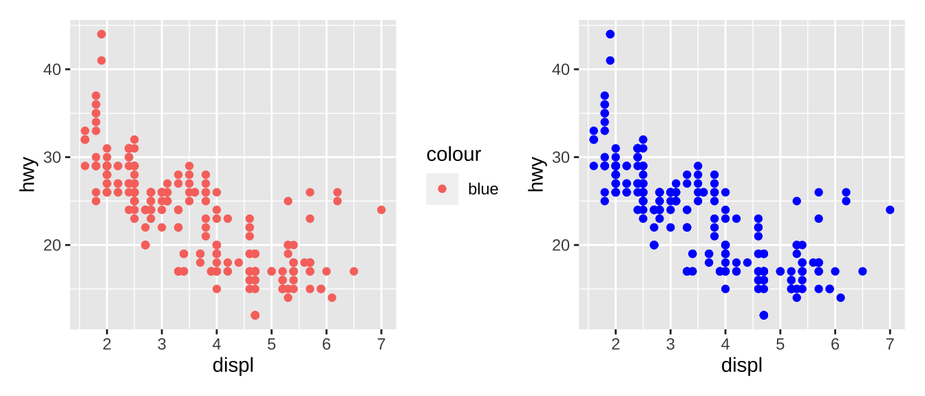
Two graphics are arranged horizontally by | (+ will do the same thing), an operator provided by the package patchwork .
2.2 Faceting
To facet a plot you simply add a faceting specification with facet_wrap(). For example, facet_wrap(~group,ncol = 1,scales="free") will show different groups in tables of graphics using different scales, arranged in one column.
2.3 Plot geoms
There are many geom functions other than geom_point(), here are some examples:
geom_smooth()fits a smoother to the data and displays the smooth and its standard error (can be turned off withgeom_smooth(se = FALSE)).method = "loess", the default for small n, uses a smooth local regression.method = "gam"fits a generalized additive model.method = "lm"fits a linear model, giving the line of best fit.method = "rlm"works likelm(), but uses a robust fitting algorithm so that outliers don’t affect the fit as much.
geom_boxplot(),geom_jitter(), andgeom_violin()produce plot to summarize the distribution of a set of points.geom_histogram()andgeom_freqpoly()show the distribution of continuous variables.geom_bar()shows the distribution of categorical variables.geom_path()andgeom_line()draw lines between the data points. However,geom_pathconnect points in the order of presentation.
More functions can be found in the cheatsheet.
2.4 Modifying the axes
The x- and y-axis labels can be modified by xlab() and ylab(). The limits of axes are controlled by xlim() and ylim(). Changing the axes limits sets values outside the range to NA. For continuous scales, use NA to set only one limit. Setting ylim inside coord_cartesian() will leave data unchanged.
# There are two ways of zooming the plot display:
# with scales or with coordinate systems.

p <- ggplot(mtcars, aes(disp, wt)) +
  geom_point() +
  geom_smooth()
p |

# Setting the limits on a scale converts
# all values outside the range to NA.
p + scale_x_continuous(limits = c(325, 500)) |

# Setting the limits on the coordinate system
# The data is unchanged, and show a portion of it
# Note how smooth continues past the points visible.
p + coord_cartesian(xlim = c(325, 500))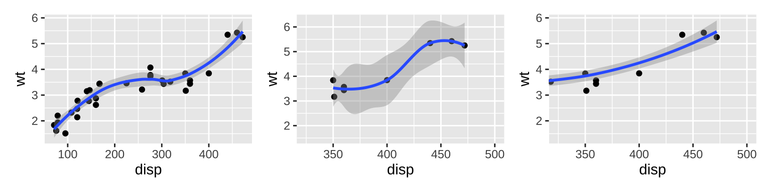
2.5 Output
There are a few things you can do with a plot object:
- Render it on screen with
print(). - Save it to disk with
ggsave(). For example, useggsave("plot.png", p, width = 5, height = 5)to save plot as png. - Briefly describe its structure with
summary(). - Save a cached copy of it to disk, with
saveRDS(). This saves a complete copy of the plot object, so you can easily re-create it withreadRDS().