1 Contrast Mechanisms and Acquisition Techniques
Two primary types of contrast are used in MRI.
- Static contrasts
Sensitive to the type, number, relaxation, and resonance properties of atomic nuclei within a voxel. Typical static contrasts are based on density (e.g., proton density), relaxation time (e.g., T1 , T2 , T2 *), chemical concentration (e.g., glutamate produced during cerebral metabolism), and even concentrations of particular types of molecules (e.g., macromolecules). We often use images sensitive to static contrast to determine brain anatomy in fMRI experiments.
- Motion contrasts
Sensitive to the movement of atomic nuclei. Typical motion contrasts provide information about the dynamic characteristics of the protons in the brain, such as blood oxygenation in fMRI, blood flow in MR angiography, water diffusion in diffusion-weighted imaging, and capillary irrigation in perfusion-weighted imaging.
1.1 Static Contrasts
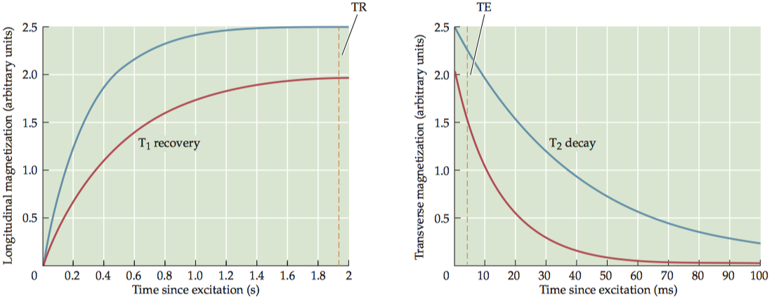
Static contrast mechanisms have been widely used in MRI thanks to their ability to illustrate basic tissue structural characteristics. There are two equations for magnetization after an initial excitation of a fully recovered spin system. \[ \left \{ \begin{array}{l} M_z(t)=M_0(1-e^{-\frac{t}{T_1}})\\ M_{xy}(t)=M_0e^{-\frac{t}{T_2}} \end{array} \right. \]
Under a short TR (The time interval between successive excitation pulses), which is not long enough to allow full recovery of the longitudinal magnetization (\(M_0(1− e^{−TR/T1})\)), the subsequent transverse magnetization is described as
\[M_{xy}(t) = M_0(1− e^{−\frac{TR}{T_1}})e^{−\frac{t}{T_2}}\]
The echo time (TE), which is the time interval between excitation and data acquisition (defined as the time when the signal from the center of k-space is acquired). For simplicity, we can replace the term t with TE to illustrate the MR signal for an image with a given TE: \[M_{xy}(t) = M_0(1− e^{−\frac{TR}{T_1}})e^{−\frac{TE}{T_2}}\] Moreover, in MRI, we are interested in comparing MR signals from multiple tissue types. To do so, we need to measure a difference in signal between any two types of tissue, known as contrast (\(C_{AB}\)). \[C_{AB}= M_{0A}(1− e^{−\frac{TR_A}{T_1}})e^{−\frac{TE_A}{T_2}}− M_{0B}(1− e^{−\frac{TR_B}{T_1}})e^{−\frac{TE_B}{T_2}}\]
1.1.1 Proton-density contrast
Proton-density images, as the name implies, provide contrast based on the sheer number of protons in a voxel, which, of course, differs in different tissue types.
To maximize proton-density contrast, researchers use pulse sequences that minimize T1 and T2 contrasts. To minimize T1 contrast, a pulse sequence must use very long TR (e.g., three times as long as T1) to ensure full T1 recovery, and to minimize T2 contrast, a pulse sequence must use a very short TE (e.g., one-tenth as long as T2) to prevent any significant T2 decay.
One disadvantage of using a very long TR is that it greatly increases imaging time. To reduce acquisition time while still maintaining proton-density contrast, a smaller flip angle (less than 90°) may be used for excitation, to only partially tip the longitudinal magnetization toward the transverse plane.
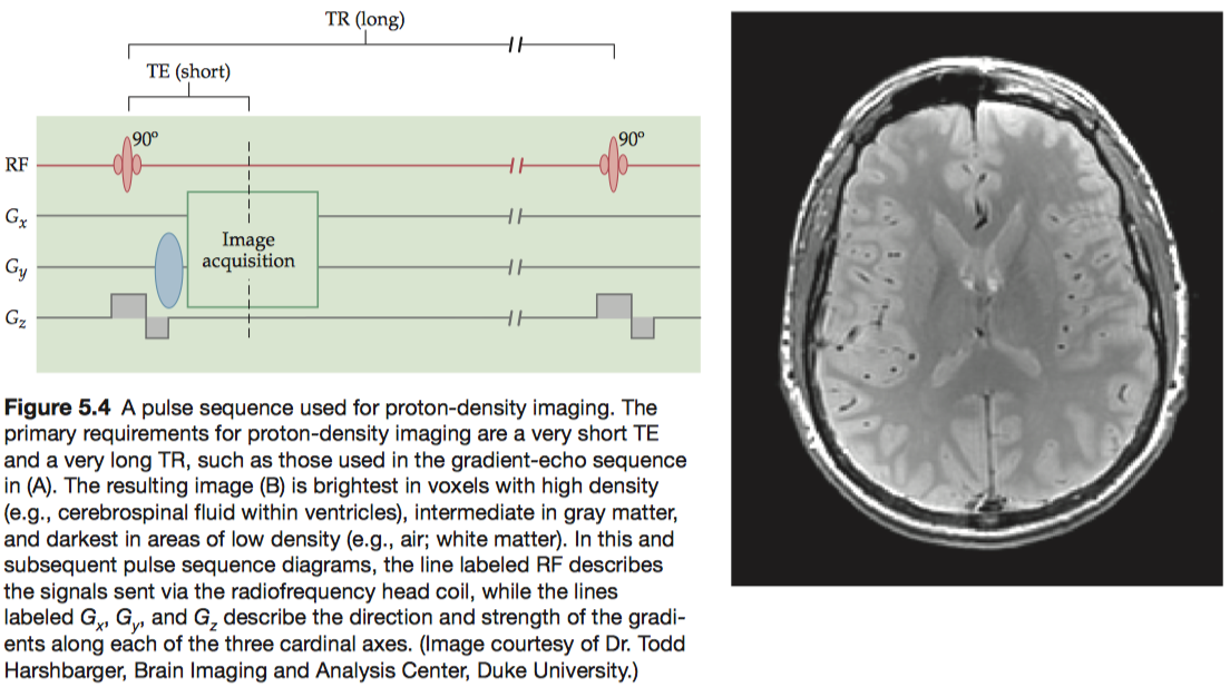
To facilitate tissue segmentation, protondensity images are frequently acquired at the same slice locations as T1 - or T2 -weighted images (see below) so that complementary anatomical information can be acquired.
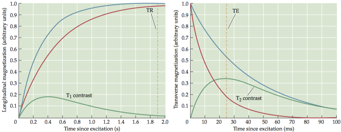
1.1.2 T1 contrast
For any two tissues that differ in T1 , there is an optimal TR value that maximally differentiates between them. To have exclusive T1 contrast, we must also have a very short TE in order to minimize T 2contrast. Note that the proton density of the tissues always contributes to the contrast, because the number of spins in the imaging volume determines the original net magnetization.
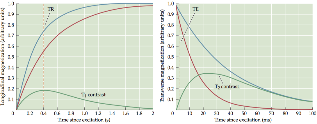
Images of T 1contrast elicit the most signal from white matter and bone marrow, due to their short T1 values, and an intermediate amount of signal from gray matter.
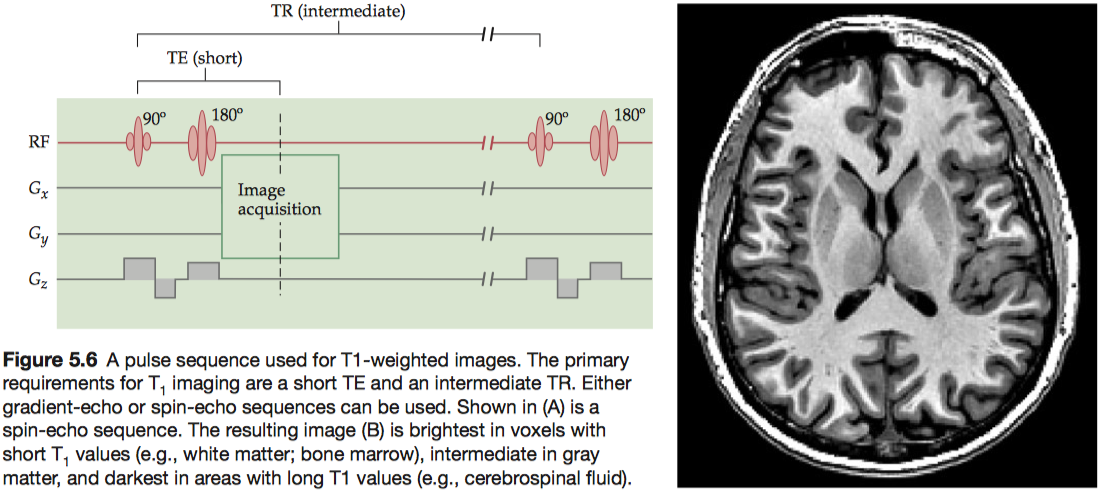
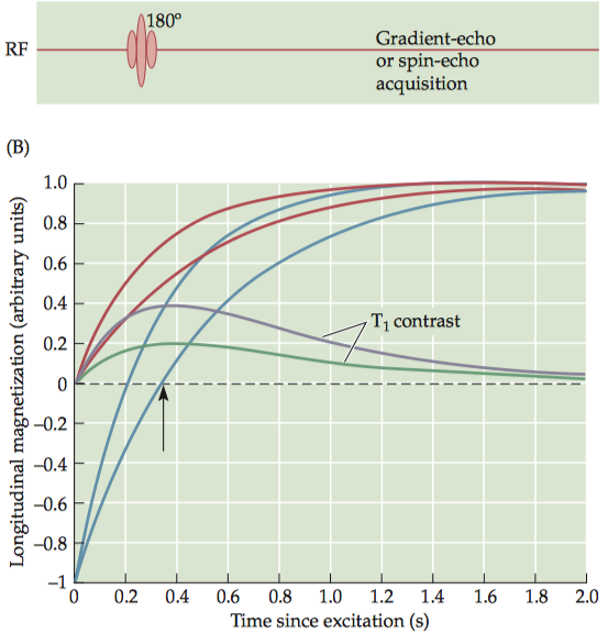
To boost T1 contrast, researchers often use a technique called inversion recovery, which begins the sequence with a 180° inversion pulse rather than the more common 90° pulse. Because the inversion pulse flips the net magnetization to the negative state, it effectively doubles the dynamic range of the signal.
1.1.3 T2 contrast
To have exclusive T2 contrast, we must have a very long TR so that the longitudinal recovery is almost complete and T1 contrast is minimal. At an intermediate TE, the difference in transverse magnetization can be maximized.
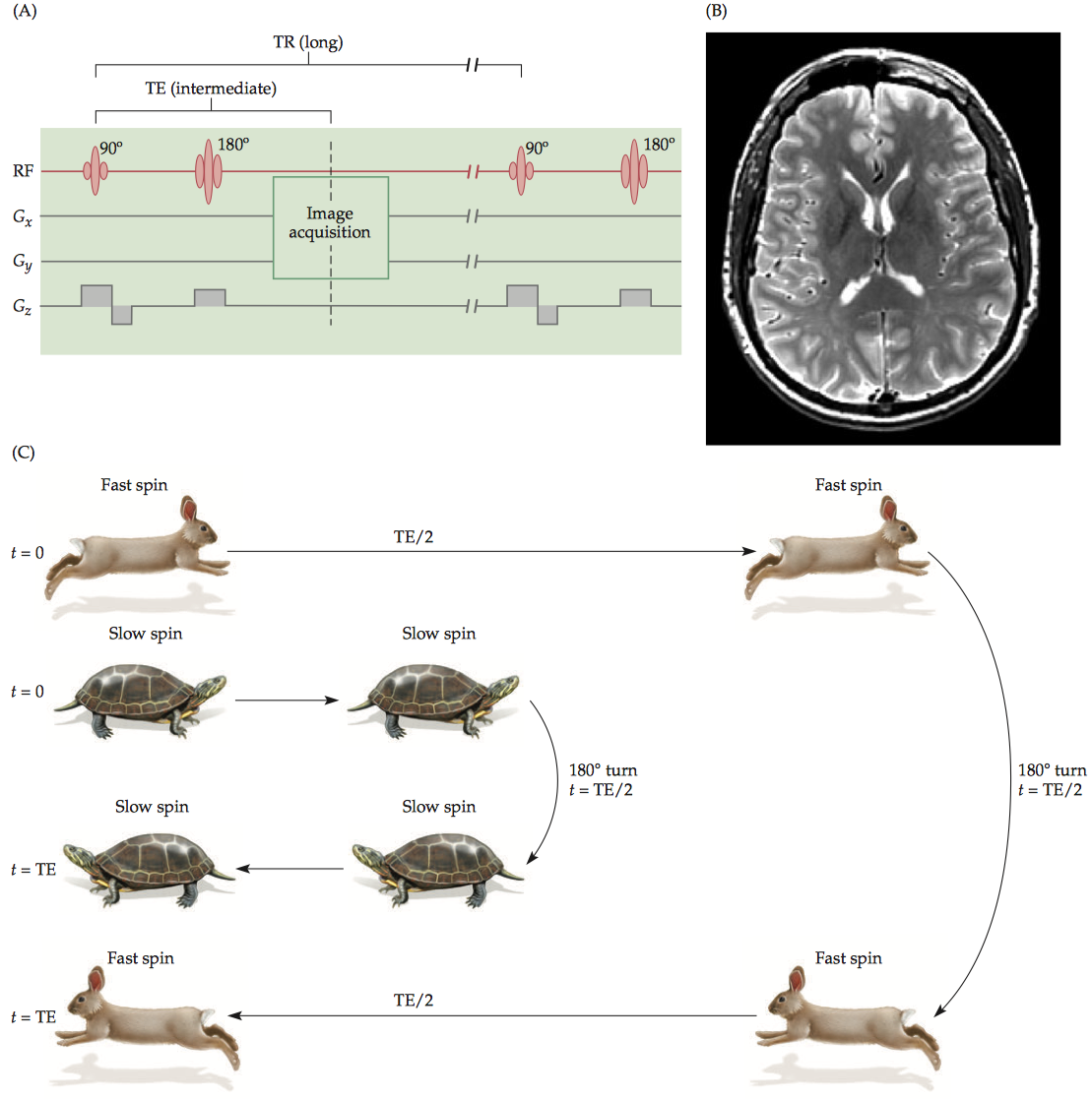
T2-weighted images can only be generated using spin-echo-based pulse sequences because only SE sequences allow true spin–spin relaxation that does not depend on the field inhomogeneity.
T2 values depend on spin–spin interactions; thus, homogeneous tissues tend to have longer T2 relaxation periods than other regions.(CSF > gray matter > white matter).
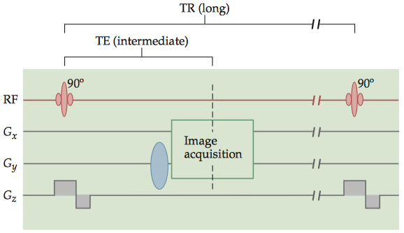
1.1.4 T2* contrast
Quantitatively, the relationship between T2 and T2* is given by 1/T2* = (1/T2 ) + (1/T2ʹ), where T2 ʹ reflects the dephasing effect caused by field inhomogeneity. Like T2 contrast, T2* contrast is provided by pulse sequences with long TR and intermediate TE values. An additional requirement is that the pulse sequence must use magnetic field gradients (and GRE pulse sequences) to generate the signal echo.
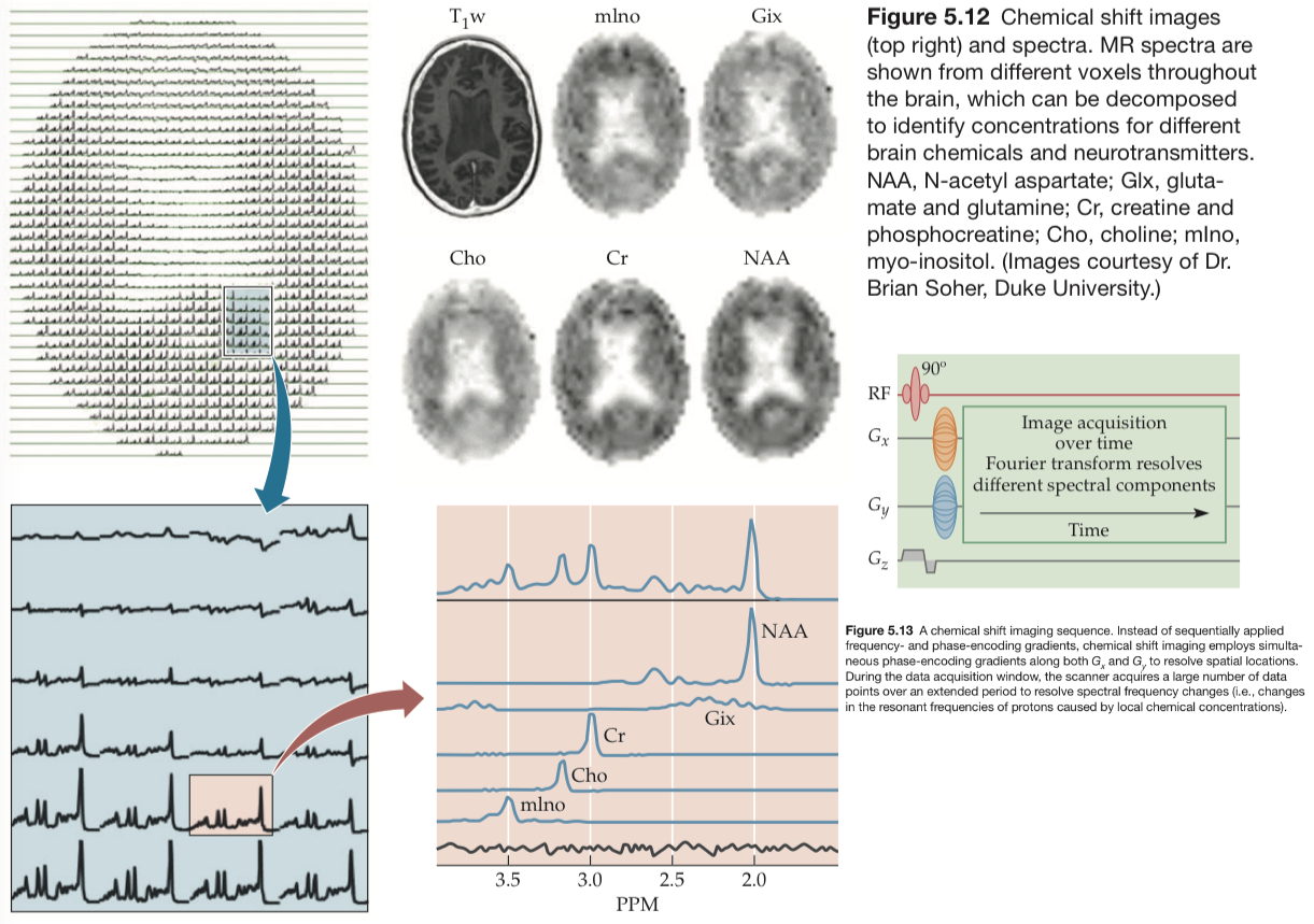
1.1.5 Chemical contrast
An important technique used to measure these substances is called chemical shift imaging. The chemical shift reflects the difference in proton resonance frequencies in different molecules.
1.2 Motion Contrasts
- Structural techniques
- MR angiography-neurovascular system
- Diffusion tensor imaging-white-matter tracts
- Functional techniques
- Dynamic diffusion imaging-water molecules
- Perfusion imaging-blood flow
1.2.1 MR angiography
For a typical contrastenhanced MRA, a small quantity (or bolus) of a gadolinium-based contrast agent is injected into the patient’s bloodstream. The gadolinium itself is not visible on MR images, but it radically shortens the T 1 recovery period for nearby blood, allowing the use of specialized pulse sequences with extremely short TRs (3 to 7 ms) and TEs (1 to 3 ms).
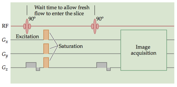
There are two primary techniques for endogenous, contrast MRA. The most common is time-of-flight (TOF) MRA. By repeatedly and frequently applying excitation pulses (SE) or gradient pulses (GRE) to a single imaging plane, the signal within that plane can be suppressed (spin satuation). Thus, tissues whose spins remain within the plane, such as gray or white matter, will produce little MR signal. Blood vessels, however, are constantly replenished with new spins from outside the plane, which contribute normal levels of MR signal. The TR and slice thickness of a TOF image must be chosen based on the expected flow.
The imaging plane is presaturated by the electromagnetic excitation pulse and gradient saturation pulses. After a brief waiting period during which fresh blood can enter the plane, the MR signals are acquired by a GRE acquisition technique, so that only the signal from this new blood will be present.
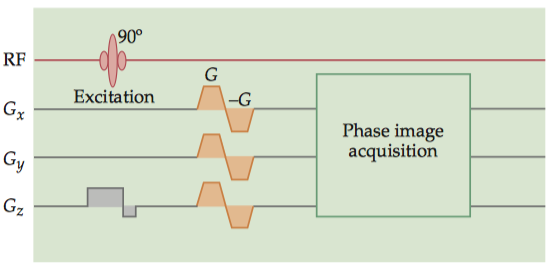
A second technique is velocity-encoded phase RF contrast (VENC-PC) MRA, which uses gradient fields to produce a difference in precession phase between the vasculature and the surrounding tissue. Typical VENC-PC protocols involve the acquisition of two sets of images: one with a strong gradient and the other with either no gradient or a gradient in the opposite direction. The difference between these images indicates the magnitude of the phase difference at each voxel, so the brightness at each voxel is proportional to flow.
1.2.2 Diffusion-weighted contrast
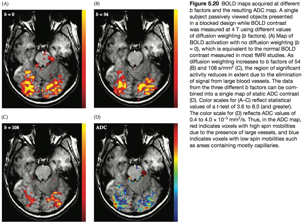
Diffusion weighting is the application of controlled gradient magnetic fields to quantify the amplitude and direction of diffusion. The attenuation effect (A) due to diffusion weighting (assuming a constant amplitude for the diffusion weighting gradient) is given by the exponential \[A=e^{-bD}=e^{-D∫_0^T [ γ G(t)t ]^2 dt}\] where D is the apparent diffusion coefficient (ADC) (i.e., the measured value of the diffusion coefficient), G is the strength of the diffusion-weighting gradient, and T is the duration of the diffusion-weighting gradient.
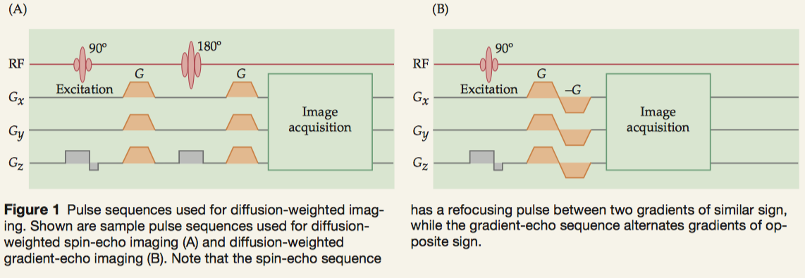
To determine the coefficients of diffusion along different directions (i.e., axes of a diffusion tensor), we need to apply controlled gradients in a pulse sequence. These gradients must be balanced in time to preserve the MR signal.
- spin-echo sequences: presenting the gradients before and after the refocusing pulse.
- gradient-echo sequences: successive positive and negative gradients.
A particularly important form of diffusion-weighted imaging is diffusion tensor imaging (DTI), which quantifies the relative diffusivity of water in a voxel into directional components. Tractography is an advanced application of DTI.
A scalar quantity known as fractional anisotropy (FA) can be computed for each voxel to express the preference of water to diffuse in an isotropic or anisotropic manner. FA values are bounded by 0 (water molecules are equally likely to diffuse in any direction) and 1 (nearly all the water molecules in the voxel are diffusing along the same preferred axis) and are calculated as \[FA=\dfrac{\sqrt{(Dx-Dy)^2+(Dy-Dz)^2+(Dz-Dx)^2}}{\sqrt{2(Dx^2+Dy^2+Dz^2)}}\] where Dx, Dy, and Dz represent the diffusivity along the three principal axes of the diffusion tensor.
1.2.3 Perfusion-weighted contrast
The irrigation of tissues via blood delivery is known as perfusion, and the family of imaging procedures that measure this process is known as perfusion MRI. In the human brain, gray-matter perfusion is approximately 60 mL/100 g/min; white-matter perfusion is lower, about 20 mL/100 g/min. Perfusion MRI is used most frequently to generate images of blood flow in capillaries and other small vessels.
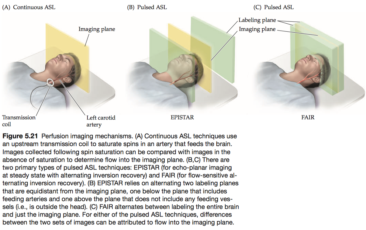
Arterial spin labeling (ASL) is a family of perfusion imaging techniques that measures blood flow by labeling spins with excitation pulses and then waiting for the labeled spins to enter the imaging plane before data acquisition.
- continuous ASL:
A type of perfusion imaging that uses a second transmitter coil to label spins within an upstream artery while collecting images. - pulsed ASL:
A type of perfusion imag-ing that uses a single coil both to label spins in one plane and to record the MR signal in another plane, separated by a brief delay period.- EPISTAR: directionally specific, in that it is only sensitive to spins flowing from the labeling plane to the imaging plane.
- FAIR: not directionally specific.
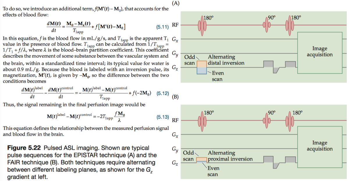
Regardless of the ASL method used, labeling blood only alters the longitudinal magnetization. Thus, we can describe the endogenous perfusion signal quantitatively by modifying the T1 term of the Bloch equation.
1.3 Image Acquisition Techniques
In this section, we will unpack the image acquisition process—also known as “filling k-space”—to form a complete description of the imaging process.
1.3.1 Echo-planar imaging
In 1976, Mansfield (Peter Mansfield, the University of Nottingham) proposed a new method, known as echo-planar imaging (EPI), in which the entire k-space is filled using rapid gradient switching following a single excitation. For this technique, Mansfield shared the Nobel Prize in Physiology or Medicine in 2003.
To fill k-space, EPI uses an unconventional pattern in which alternating lines are scanned in opposite directions.
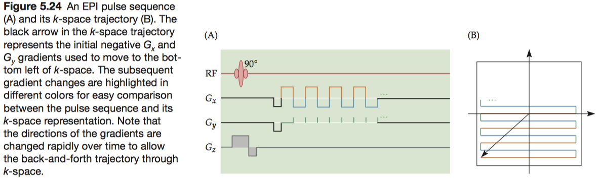
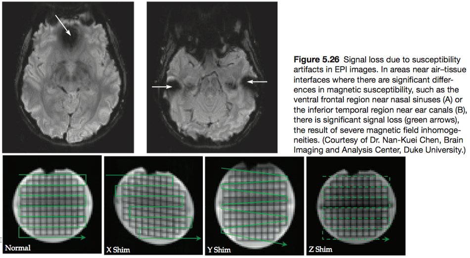
The most common EPI artifacts result from imperfections in the magnetic fields, either static or gradient, used to collect the images. Small- and large-scale static field inhomogeneities can result in signal losses and geometric distortions, respectively.
1.3.2 Spiral imaging
Compared with EPI sequences, spiral imaging sequences can be much less taxing on a gradient system and can reduce the time needed to collect an image.
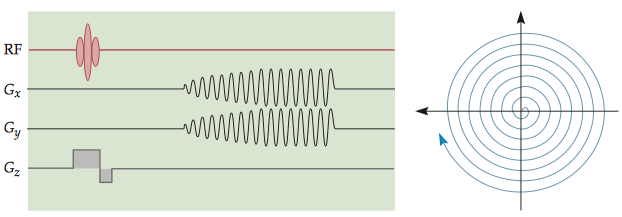
The types of spatial distortion, however, are quite different from those found in EPI. Because of the non-Cartesian k-space sampling scheme, the regular distortion pattern seen in EPI images is usually not present in spiral images.
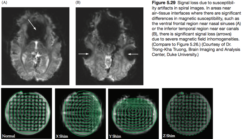
1.3.3 Signal recovery and distortion correction for EPI and spiral images
There are three types of compensation methods, all involving the shimming of the magnetic field.
- Active local shims
- Pulse sequence incorporating a gradient along the z direction
- Magnetic field map
1.3.4 Parallel imaging
If the pursuit of higher magnetic fields has been the engine advancing MRI technology, the development of parallel imaging (also known as multi-channel imaging) using large coil arrays has provided the high-octane fuel. Multiple-channel acquisition provides two major advantages.
- Increases the spatial resolution without increasing acquisition time
- Reduces the duration of the readout window, thereby improving the imaging speed and minimizing the spatial distortion.
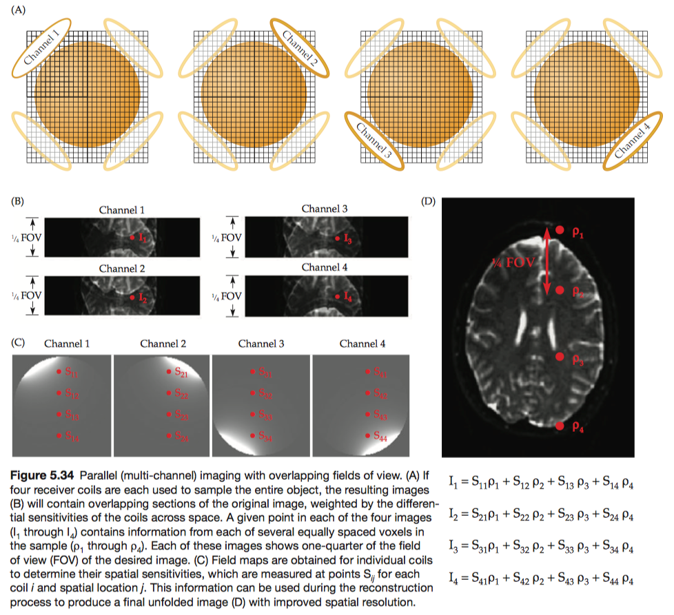
Here we use a four-coil array as an example. During the imaging session, all channels acquire data with a lower sampling density in k-space than will be used for the final image, resulting in a smaller field-of-view and four severely wrapped images.
Each voxel in these images contains signal from four overlapping images of the brain. The intensity of any given voxel in each of these four images, \(I_1\) to \(I_4\) , reflects a combination of the sensitivity \(S_{ij}\) (can be identified from field maps) of each coil i at that location j and the actual intensity values for that voxel in each of the images (\(ρ_1\) through \(ρ_4\)).
In addition to increasing spatial resolution, multiple-channel acquisition can also be used to increase the raw SNR. When multiple coils are targeted at the same brain region, images from individual channels can be combined to increase the magnitude of the signal.
Parallel imaging can also improve temporal resolution without sacrificing spatial resolution or spatial coverage. Note that the addition of coils has different effects on spatial and temporal resolution. Because spatial resolution is measured in squared units within a slice (\(\mathrm{mm}^2\)), it increases in proportion with the change in the square root of the number of coils. But temporal resolution is measured in linear units (seconds), and it improves linearly with the number of coils.