1.1.1 Longitudinal magnetization (\(M_z\))

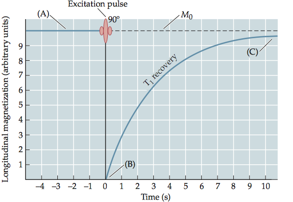
The magnitude of the longitudinal magnetization (\(M_z\)) depends only on a single first-order differential equation. Thus, its solution is an exponential recovery function that describes the return of the main magnetization to the original state. We assume that the initial magnetization at time zero is given by \(M_{z0}\), \[ \begin{aligned} &\quad\qquad\dfrac{\mathrm{d}{M_z}}{\mathrm{d}t}={}-\dfrac{(M_z-M_0)}{T_1}\\ &\Rightarrow \quad\dfrac{\mathrm{d}{(M_z-M_0)}}{\mathrm{d}t}={}-\dfrac{(M_z-M_0)}{T_1}\\ &\Rightarrow \quad\dfrac{\mathrm{d}{(M_z-M_0)}}{(M_z-M_0)}={}-\dfrac{\mathrm{d}t}{T_1}\\ &\Rightarrow \quad\ln(M_z(t)-M_0)\Big|_0^{t'}={}-\dfrac{t}{T_1}\Big|_0^{t'}\\ &\Rightarrow \quad M_z=M_0+(M_{z0}-M_0)e^{-\frac{t}{T_1}} \end{aligned} \] To illustrate \(T_1\) recovery, let’s consider some extreme values for the initial magnetization, \(M_{z0}\). Consider the situation in which the net magnetization is fully relaxed. Here, \(M_{z0}\) is equal to \(M_0\) , so that \(M_{z0}\) will not change. After an excitation pulse is applied, the net longitudinal magnetization is zero. The subsequent recovery of longitudinal magnetization is given by \(M_z=M_0(1-e^{-\frac{t}{T_1}})\).

1.1.2 Transverse magnetization (\(M_{xy}\))

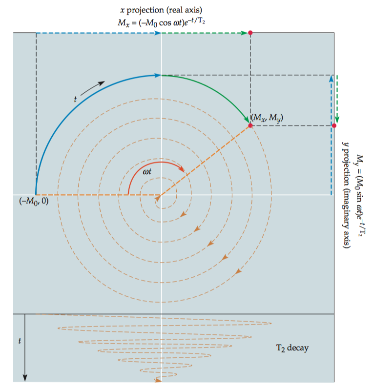
Solving for \(M_x\) and \(M_y\), given an initial magnetization of \((M_{x0} ,\ M_{y0})\), we get the equation pair \[ \left \{ \begin{array}{l} M_x=(M_{x0}\cos ωt+M_{y0}\sin ωt)e^{-\frac{t}{T_2}}\\ M_y=(-M_{x0}\sin ωt + M_{y0}\cos ωt )e^{-\frac{t}{T_2}} \end{array} \right. \] We can combine the x and y components of the net magnetization into a more generalized single quantity, \(M_{xy}\) , which represents the transverse magnetization. The quantity \(M_{xy}\) is traditionally represented as a complex number. \[M_{xy}=M_x+iM_y\] For an arbitrary initial magnitude of the transverse magnetization \(M_{xy0} = M_{x0} + iM_{y0}\) , the transverse magnetization can be represented as: \[ \begin{aligned} M_{xy}&=(M_{x0} + iM_{y0})e^{-\frac{t}{T_2}}(\cos ωt-i\sin ωt)\\ &=M_{xy0}e^{-\frac{t}{T_2}}e^{-i \omega t} \end{aligned} \]

After excitation, spins experience a magnetic field, B, that depends on the large static field, B0, and the smaller gradient field, G. Note that, the direction of B is always aligned with the main field. Therefore, we can describe the magnitude of the total magnetic field (B) experienced by a spin system at a given spatial location (x, y, z) and time point (t) as a linear combination of the static field and gradient fields. \[B(\tau)=B_0+G_x(\tau)x+G_y(\tau)y+G_z(\tau)z\] Knowing that \(\omega = \gamma B\), we can substitute the \(\omega\) term in previous equation using the magnitude of the total magnetic field described currently. \[M_{xy}(x,y,z,t) = M_{xy0}(x,y,z)e^{-\frac{t}{T_2}}e^{−iγB_0t}e^{−iγ\int_0^t (G_x(\tau)x+G_y(\tau)y+G_z(\tau)z) \mathrm{d}\tau}\] It states that the transverse magnetization for a given spatial location and time point, \(M_{xy} (x, y, z, t)\), is governed by four factors:

1. the original magnetization at that spatial location, \(M_{xy0}(x,y,z)\);
2. the signal loss due to \(e^{-\frac{t}{T_2}}\);
3. the accumulated phase due to the main magnetic field, \(e^{−iγB_0t}\);
4. the accumulated phase due to the gradient fields, which can be expressed as \[e^{−iγ\int_0^t (G_x(\tau)x+G_y(\tau)y+G_z(\tau)z) \mathrm{d}\tau}\]

1.1.3 The MR signal equation

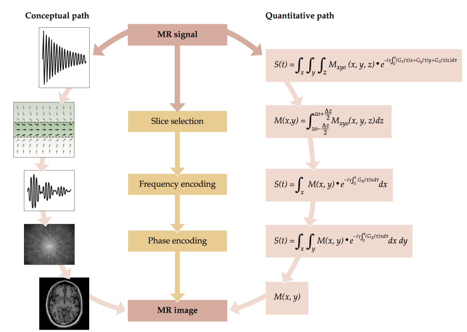
The MR signal measured by that antenna reflects the sum of the transverse magnetizations of all voxels within the excited sample. This can be restated in the formal mathematical terms, which expresses the MR signal at a given point in time, \(S_{(t)}\), as the spatial summation of the MR signal from every voxel. \[S(t)=\int_x\int_y\int_zM_{xy}(x,y,z,t)\mathrm{d}x\mathrm{d}y\mathrm{d}z\] Combining with previous equation results in \[S(t) = \int_x\int_y\int_zM_{xy0}(x,y,z)e^{-\frac{t}{T_2}}e^{−iγB_0t}e^{−iγ\int_0^t (G_x(\tau)x+G_y(\tau)y+G_z(\tau)z) \mathrm{d}\tau} \mathrm{d}x \mathrm{d}y \mathrm{d}z\] This vastly important equation is known as the MR signal equation because it reveals the relationship between the acquired signal, \(S(t)\), and the properties of the object being imaged, \(M (x, y, z)\).

In practice, the term \(e^{−i γω_0 t}\) is not necessary for calculation of the MR signal, because modern MRI scanners demodulate the detected signal with the resonance frequency \(\omega_0\). That is, they synchronize data acquisition to the resonance frequency, which is analogous to the idea of transforming from laboratory to rotating reference frames.The \(T_2\) decay term, \(e^{−\frac{t}{T_2}}\), affects the magnitude of the signal but not its spatial location, so we can ignore it for the moment and arrive at a simpler version of the MR signal equation. \[S(t) = \int_x\int_y\int_zM_{xy0}(x,y,z)e^{−iγ\int_0^t (G_x(\tau)x+G_y(\tau)y+G_z(\tau)z) \mathrm{d}\tau} \mathrm{d}x \mathrm{d}y \mathrm{d}z\] In principle, we can collect a single 3-D MR image by systematically turning on gradient fields along the x, y, and z-axes. However, because 3-D imaging sequences present addtional technical challenges and are less tolerant of hardware imperfections than other methods, most forms of imaging relevant to fMRI studies use two-dimensional imaging sequences.

1.2.1 Slice selection

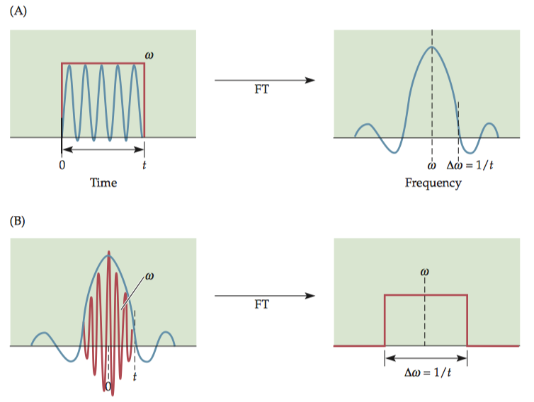
Since the Fourier transform of a sinc function is a rectangular function, a sincmodulated pulse has a rectangular frequency response; thus, it contains all frequencies within a rectangular band and no frequencies outside that band.

Although a perfectly rectangular slice profile would be optimal, it is difficult to achieve because of off-resonance excitation. The primary consequence for MRI is crossslice excitation, or the bleeding of excitation from one slice to the next. If we excite adjacent slices sequentially, each slice will have been pre-excited by the previous excitation pulse, leading to saturation of the MR signal. To minimize this problem, most excitation schemes use interleaved slice acquisition.

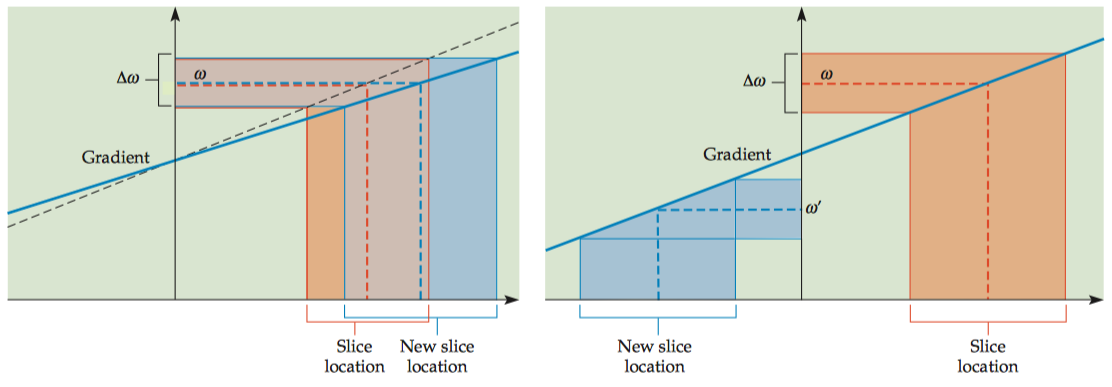
Slice location and thickness are determined by three factors:

1. The center frequency of the excitation pulse (\(\omega\))
2. The frequency bandwidth of the excitation field (\(Δ\omega\))
3. The strength of the gradient field (\(G_z\))

By changing the slope of the gradient, the same radiofrequency pulse can be used to select a slice with a different location and thickness. By changing the center frequency of the excitation pulse to \(\omegaʹ\), the same gradient can be used to select a different slice location.

For a given location (x, y) within a slice, the total magnetization summed along the z direction, M(x, y), for a thickness Δz and center \(z_0\) is given by \[M(x,y)=\int_{z_0-\frac{Δz}{2}}^{z_0+\frac{Δz}{2}} M(x,y,z) \mathrm{d}z\] After slice selection, all signals along the z direction are integrated, so the magnetization, M, is dependent only on x and y, but not on z. \[S(t) = \int_x\int_yM_{xy0}(x,y)e^{−iγ\int_0^t (G_x(\tau)x+G_y(\tau)y) \mathrm{d}\tau} \mathrm{d}x \mathrm{d}y\]

1.2.2 Frequency and phase encoding

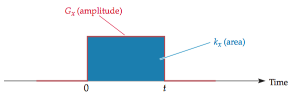
Consider the terms \(k_x\) and \(k_y\) given in the following equations, where each equation represents the time integral of the appropriate gradient multiplied by the gyromagnetic ratio: \[ \left \{ \begin{array}{l} k_x(t)=\dfrac{\gamma}{2\pi}\int_0^t G_x(\tau)\mathrm{d}\tau\\ k_y(t)=\dfrac{\gamma}{2\pi}\int_0^t G_y(\tau)\mathrm{d}\tau \end{array} \right. \] These equations state that changes in k-space over time, or k-space trajectories, are given by the time integrals of the gradient waveforms. In other words, the k-space trajectories are simply the areas under the gradient waveforms.

By substituting these terms into previous equation, we can restate the MR signal equation using k-space coordinates as \[S(t)=\int_x\int_yM(x,y)e^{−i 2\pi k_x(t)x} e^{-i 2\pi k_y(t)y} \mathrm{d}x \mathrm{d}y\] It indicates that k-space and image space have a straightforward relationship: they are 2-D Fourier transforms of each other. A inverse Fourier transform can convert k-space data into an image, a process known as image reconstruction. Conversely, a forward Fourier transform can convert image-space data into k-space data.

Because a complete sample of the k-space is usually required to construct an image, collecting the MR signal is often referred to as filling k-space. In some anatomical imaging sequences, like the gradient-echo (GRE) imaging sequence, k-space is filled one line at a time, following g a succession of individual excitation pulses.

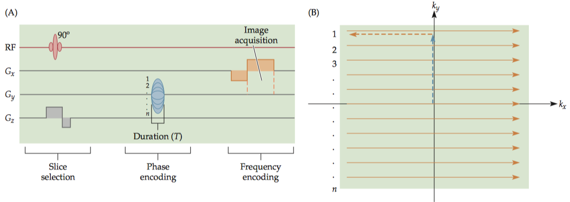
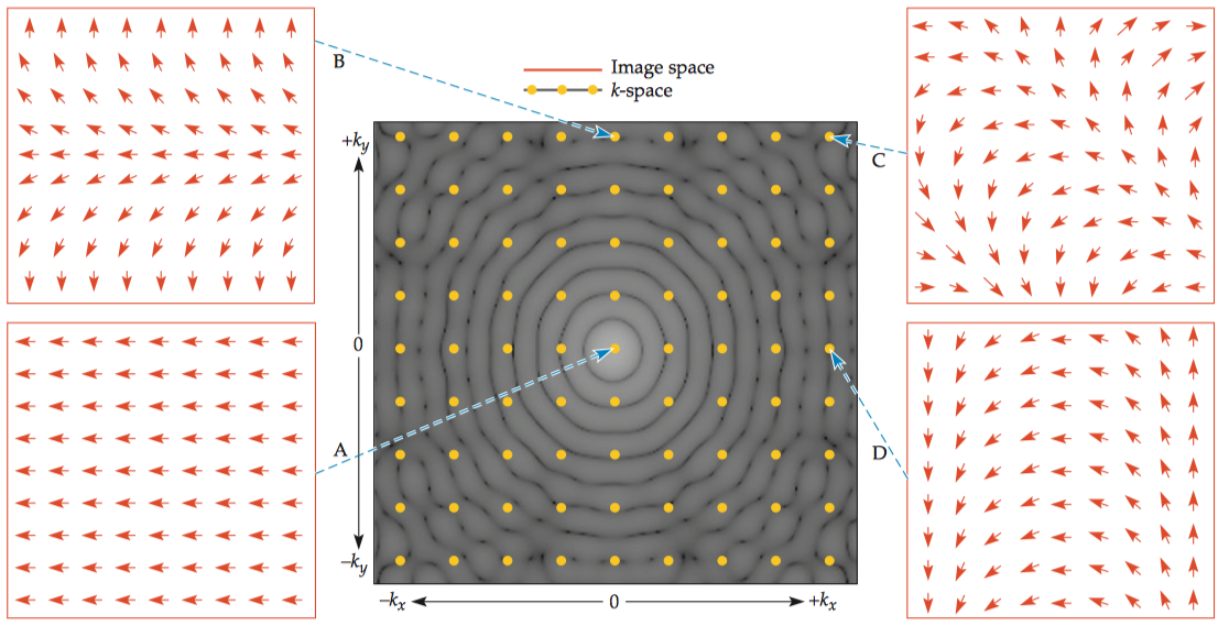
The phase-encoding gradient \(G_y\) over time \(T\) changes the \(k_y\) value and results in the movement of the k-space trajectory in the amount of \(\dfrac{\gamma G_y T}{2π}\), along the y direction, as shown by the blue arrow. On the actual MR signal, the phase-encoding process adds a modulation term \(e^{−i\gamma G_y T \cdot y}\) \[S(t)=\int_y M(x,y) e^{−i\gamma G_y T \cdot y} \mathrm{d}y\] After the phase-encoding step, the frequency-encoding gradient changing the frequency of the spins at a given location along x. At a given time t changes the k xvalue and results in the movement of the k-space trajectory in the amount of \(\frac{\gamma G_x t}{2π}\), along the x direction as indicated by orange arrows \[S(t)=\int_x\int_y M(x,y) e^{−i 2\pi k_x(t) \cdot x} e^{−i\gamma G_y T \cdot y} \mathrm{d}x\mathrm{d}y\] In the case of phase encoding, we can increment the amplitude of \(G_y\) to change \(k_y\) and step along the y direction in the k-space (because T is fixed); in the case of frequency encoding, we can actually keep the same \(G_x\) amplitude; just let the increment in time change \(k_x\), and step along the x direction in the k-space.

Although the trajectory along the \(k_x\) direction is continuous, the MR signal is sampled digitally with a specific interval, so each row consists of a number of discrete data points.

1.2.3 Relationship between image space and k-space

k-space reflects the spatial frequency of the object(s) in the image space. The image below shows two circles, one offset from the center. If we trace a line from the top left to the bottom right of the image, it will encounter two circles separated by a distance between their centers. The k-space data will thus have a spatial-frequency component along that line, with the frequency equal to the inverse of that distance. This component is visible as a grating running from top left to bottom right in the k-space image, on top of the concentric pattern that results from the shapes of the circles.

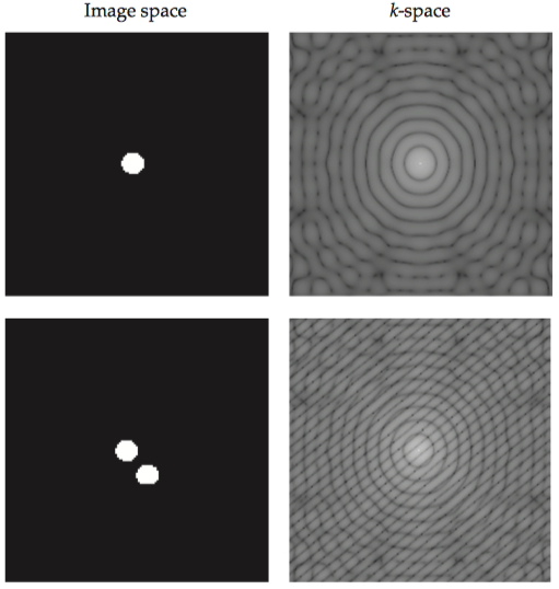
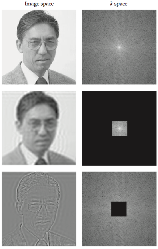
The k-space image is brightest in the center and darkest near the edges, which illustrates that low-spatial-frequency data (i.e., grating patterns with thick lines) from near the center of k-space are most important for determining the signal-to-noise ratio of the image.

Contrary to intuition, there is not a one-to-one relationship between points in k-space and voxels in image space. For the point at the center of k-space, all the magnetization vectors are at the same phase, and thus the total signal is at its maximum. At other k-space points, the magnetization vectors differ across voxels, and the intensity of the k-space point represents the sum of those vectors.

1.2.4 Converting from k-space to image space

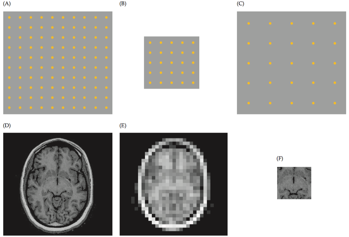
After k-space is filled, a 2-D inverse Fourier transform is necessary for conversion of the raw data from k-space to image space, M(x, y). In image space, the basic sampling unit is distance; in k-space, the basic sampling unit is spatial frequency (1/distance). Conversely, finer sampling in k-space results in a greater extent of coverage, or a larger field of view, in the image domain.

Here, field of view (FOV) is defined as the total distance along a dimension of image space (i.e., how large the image is), or \[ \left \{ \begin{array}{l} \mathrm{FOV}_x=\dfrac{1}{\Delta k_x}=\dfrac{1}{2\pi\gamma(G_x\Delta t)}=\mathrm{sampling\ rate\ along\ } k_x\\ \mathrm{FOV}_y=\dfrac{1}{\Delta k_y}=\dfrac{1}{2\pi\gamma(\Delta G_y T)}=\mathrm{sampling\ rate\ along\ } k_y \end{array} \right. \] Therefore, voxel size is just the FOV divided by the number of samples: \[ \left \{ \begin{array}{l} \dfrac{\mathrm{FOV}_x}{M_x}=\dfrac{1}{M_x \Delta k_x}=\dfrac{1}{2\Delta k_{x\mathrm{max}}}\\ \dfrac{\mathrm{FOV}_y}{M_y}=\dfrac{1}{M_y \Delta k_y}=\dfrac{1}{2\Delta k_{y\mathrm{max}}} \end{array} \right. \] Note that the quantities \(2k_{x\mathrm{max}}\) and \(2k_{y\mathrm{max}}\) refer to the total extent of k-space along each of the cardinal directions. If \(k_\mathrm{max}\) is large, the voxel size will be small. Decreasing the separation between adjacent data points in k-space increases the FOV in image space. Likewise, increasing the extent of k-space decreases the voxel size in image space. Note also that if we want to collect data from N × N voxels in our image, we need an equal number of k-space data points (N × N data points).

1.4.1 Inhomogeneity of the static magnetic field

Note that inhomogeneity in the static magnetic field becomes increasingly problematic at higher field strengths, because it becomes more difficult to adequately shim the field to correct for local distortions. The imperfection in the static field can be mathematically represented by a difference quantity, \(ΔB_0\) , representing the increased or decreased field strength at a given location. \[S(t)=\int_x\int_y M(x,y) e^{−i 2\pi (k_x(t) \cdot x + k_y(t) \cdot y+\Delta B_0\cdot t)} \mathrm{d}x\mathrm{d}y\] In practice, field inhomogeneities can lead to two distinct types of artifacts:

1. geometric distortions

Because the frequency of spins depends on the magnetic field strength, these inhomogeneities will lead to changes in spin frequencies. Remember that the position of a voxel is encoded by its frequency. Thus, a voxel with the incorrect resonant frequency will be displaced to an incorrect spatial location.

2. signal losses

When there is a long time between the slice excitation and signal readout (e.g., to reach sufficient \(T_2^*\) contrast in a fMRI study), magnetic field inhomogeneities can cause spins within a voxel to accumulate different amount of phase, leading to interference and the loss of MR signal.

1.4.2 nonlinearities in the gradient fields

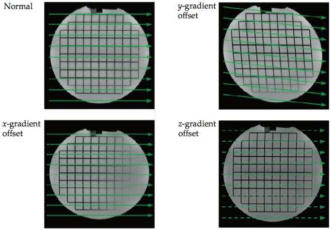
Depending on the pulse sequences and their distinct k-space trajectories, the nonlinearities in the gradient fields will be manifested differently. Here we use an example to illustrate these artifacts using a typical gradient-echo pulse sequence.

1. If the x-gradient \(G_x\) is off by a small amount, the resulting k-space trajectories will have an error along the \(k_x\) direction.
2. If the y-gradient \(G_y\) is off, the k-space trajectories will be skewed along the \(k_y\) direction. Note that this skew affects both the onset of each line in k-space as well as the path taken through k-space. The magnitude of this skew depends on the time integral of the gradient amount.
3. If the z-gradient \(G_z\) is off, the slope of the excitation gradient will be altered, leading to changes in slice thickness and signal intensity, but the shape of the object would not be distorted.