- 1 MR Signal Generation
- 1.1 Magnetic Moment
- 1.2 Angular Momentum
- 1.3 Spins in an External Magnetic Field
- 1.4 Energy Difference between Parallel and Antiparallel States
- 1.5 Magnetization of a Spin System
- 1.6 Excitation of a Spin System and Signal Reception
- 1.7 Relaxation Mechanisms of a Spin System
- 1.8 The Bloch Equation for MR Signal Generation
- 2 Basic Principles of MR Image Formation
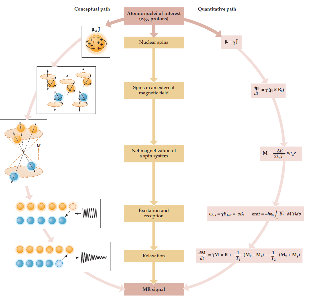
1 MR Signal Generation
1.1 Magnetic Moment
Consider a simple rectangular current loop of length (L) and width (W). Magnetic moment µ is defined as the maximum torque divided by the magnetic field strength (B). The maximum torque exerted by the magnetic field when it is perpendicular to the rectangular current is given by multiplying the maximum force exerted on the current element by its width.
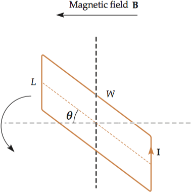
\[\vec\mu=\dfrac{\vec\tau_{max}}{\vec{B}}=\dfrac{I\vec{B}LW}{\vec{B}}=IA\]
1.2 Angular Momentum
The angular momentum is defined as the product of the mass (m), the angular velocity (w), and the radius (r) squared. \[\vec{J}=m \omega r^2\] The vectors defining the current flow and rotation have the same direction, so there should exist a scalar factor between the magnetic moment and angular momentum. \[\vec\mu=\gamma\vec{J}\] To understand what g represents, let’s consider the simplest atomic nucleus, a single proton. First we must make some assumptions, namely that the charge (q) of the proton is an infinitely small point source, the proton rotates about a radius (r), and its rotation has a period (T). \[\vec\mu=IA=\frac{q}{T} \pi r^2\] \[\vec{J}=m \omega r^2=m\frac{2\pi}{T}r^2\] \[\therefore \gamma=\frac{\vec\mu}{\vec{J}}=\frac{q}{2m}\] Since the charge and mass of the proton (or any other atomic nucleus) never change, \(\gamma\) is a constant for a given nucleus, regardless of the magnetic field strength, temperature, or any other factor. The constant \(\gamma\) is known as the gyromagnetic ratio, and it is critical for MRI.
1.3 Spins in an External Magnetic Field
If we place a magnetic bar that is not spinning into a static magnetic field at an angle θ, it will oscillate back and forth across the main field. However, if the magnetic bar is spinning about its axis, it will wobble around this field instead of oscillating back and forth.
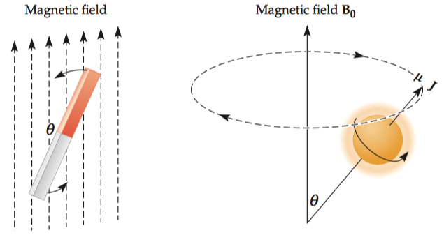
A moving charge experiences torque (\(\tau\) ) equal to the cross product of the magnitude of its magnetic moment (µ) and main field strength (\(B_0\)). \[\vec{\tau}=\vec{\mu} \times \vec{B_0}\] Since torque indicates the change in angular momentum over time, it can be defined as the derivative of angular momentum over the derivative of time. \[\vec{\tau}=\frac{\mathrm{d}\vec{J}}{\mathrm{d}t}=\frac{\mathrm{d}\vec{\mu}}{\gamma\mathrm{d}t}=\vec{\mu} \times \vec{B_0}\] \[\therefore \frac{\mathrm{d}\vec{\mu}}{\mathrm{d}t}=\gamma(\vec{\mu} \times \vec{B_0})\] We can transform this equation into three separate scalar equations, representing three different dimensions. \[ \left \{ \begin{array}{l} \dfrac{\mathrm{d}{\mu_x}}{\mathrm{d}t}=\gamma\mu_yB_0 \\ \dfrac{\mathrm{d}{\mu_y}}{\mathrm{d}t}=-\gamma\mu_xB_0 \\ \dfrac{\mathrm{d}{\mu_z}}{\mathrm{d}t}=0 \end{array} \right. \] At time zero, the components along the three directions can be defined as \(\mu_{x0}\), \(\mu_{y0}\), and \(\mu_{z0}\). The total magnetic moment, \(\vec\mu(0)\), is simply the sum of the three components. Here, \(\vec{x}\), \(\vec{y}\), and \(\vec{z}\) are unit vectors along the three cardinal directions. \[\vec\mu(0)=\mu_{x0}\vec{x}+\mu_{y0}\vec{y}+\mu_{z0}\vec{z}\] Solving the set of differential equations with given the initial conditions at time zero, we can get: \[\vec\mu(t)=(\mu_{x0}\cos ωt+ \mu_{y0}\sin ωt)\vec{x} + (\mu_{y0}\cos ωt − \mu_{x0}\sin ωt)\vec{y}+ \mu_{z0}\vec{z}\] Importantly, the angular velocity \(\omega\) is given by \(\gamma B_0\), which is the Larmor frequency.
1.4 Energy Difference between Parallel and Antiparallel States
Energy difference between the states (∆E) can be calculated by integrating the torque over the 180º rotation angle during this flip, which is also the energy emitted or absorbed in the form of an electromagnetic pulse. \[\Delta E=h\nu=\int_0^{\pi}\tau \mathrm{d}\theta =\int_0^{\pi}\mu B_0 \sin\theta \mathrm{d}\theta=-\mu B_0 \cos\theta\Big|_0^\pi=2\mu B_0\] \[\therefore \nu=\dfrac{2\mu B_0}{h}\] It was shown experimentally that the longitudinal component (i.e., along the magnetic field) of the angular momentum J of a proton is h/4π. \[\nu=\dfrac{2\mu B_0}{h}=\gamma J\dfrac{2B_0}{h}=\gamma(\dfrac{h}{4\pi})\dfrac{2B_0}{h}=\dfrac{\gamma}{2\pi}B_0\] The correspondence between \(\omega\)(rad per second) and \(\nu\) (cycle per second) means that a single quantity, the Larmor frequency, governs two aspects of a spin within a magnetic field: the energy that the spin emits or absorbs when changing energy states and the frequency at which it precesses around the axis of the external magnetic field.
1.5 Magnetization of a Spin System
In the absence of a magnetic field, the spin axes of the nuclei in bulk matter are oriented in random directions, so that the net magnetization (i.e., the sum of all individual magnetic moments) is zero. Once the bulk matter is moved into a magnetic field, each magnetic moment must align itself in either the parallel or antiparallel state. We will refer to the parallel state as p and the antiparallel state as a, and their probabilities are \(P_p\) and \(P_a\) respectively. \[P_p+P_a=1\] The relative proportion of the two spin states depends on their energy difference (∆E) and the temperature (T). This proportion can be determined using Boltzmann’s constant, \(k_B\) (1.3806 × 10 –23 J/K), which governs the probabilities of spin distribution under thermal equilibrium. \[\dfrac{P_p}{P_a}=e^{\frac{\Delta E}{Tk_B}}\] Given the very small value of Boltzmann’s constant, ∆E/T\(k_B\) will be much less than 1 under normal conditions. For very small exponents x, the exponential \(e^x\)can be approximated by 1 + x (high-temperature approximation). \[\dfrac{P_p}{P_a}\approx 1+\frac{\Delta E}{Tk_B}\] \[\therefore P_p-P_a=\dfrac{1+\frac{\Delta E}{Tk_B}}{2+\frac{\Delta E}{Tk_B}}-\dfrac{1}{2+\frac{\Delta E}{Tk_B}}=\dfrac{\Delta E}{2Tk_B+\Delta E} \approx \dfrac{\Delta E}{2Tk_B}\] Thus, the total magnetic moment, which is called the bulk magnetization or net magnetization, is simply this proportion multiplied by the number of protons per unit volume (n) multiplied by the magnetic moment of each spin in the z direction. The net magnetization is represented by the symbol \(\vec M\), where z is a unit vector in the \(\vec z\) direction \[\vec M=(P_p-P_a)n\mu_z\vec z=\dfrac{\Delta E}{2Tk_B}n\mu_z\vec z\] Although the net magnetization is initially aligned with the main magnetic field, its precession angle is 0° at equilibrium. When tipped away from this starting position by an excitation pulse, the net magnetization will precess around the main axis of the field, just like a single magnetic moment described previously. \[ \begin{aligned} \vec M(t)&=(M_{x0}\cos ωt+ M_{y0}\sin ωt)\vec{x} + (M_{y0}\cos ωt − M_{x0}\sin ωt)\vec{y}+ M_{z0}\vec{z}\\ &=M_{x0}(\vec{x}\cos ωt-\vec{y}\sin ωt) + M_{y0}(\vec{x}\sin ωt+\vec{y}\cos ωt )+ M_{z0}\vec{z} \end{aligned} \]
1.6 Excitation of a Spin System and Signal Reception
1.6.1 Spin excitation
For hydrogen, the net magnetization oscillates around the main field vector (3T) approximately 128 million times per second. Because the magnetization rotates so rapidly, it is extremely difficult to change the magnetization with a single pulse of electromagnetic energy. Instead, energy is applied at a given frequency for an extended period of time. Let’s take a backyard swing set for example. If you apply energy at the swing’s natural frequency by pushing each time the swing is in the same place, even very small pushes will help increase the velocity of the swing, and thereby increase the energy in the system. This phenomenon—where small applications of energy at a particular frequency can induce large changes in a system—is known as resonance. For similar reasons, MRI scanners use specialized radiofrequency coils to transmit an electromagnetic excitation pulse (\(B_1\)) at the spin precession (i.e., Larmor) frequency to exert torque on the spins and perturb them. \[\vec B_1 = B_1 \vec x \cos \omega t − B_1 \vec y \sin \omega t\] For clarity, we will refer to the normal frame of reference that is aligned with the magnetic field of the scanner as the laboratory frame and the frame of reference rotating at the Larmor frequency as the rotating frame。
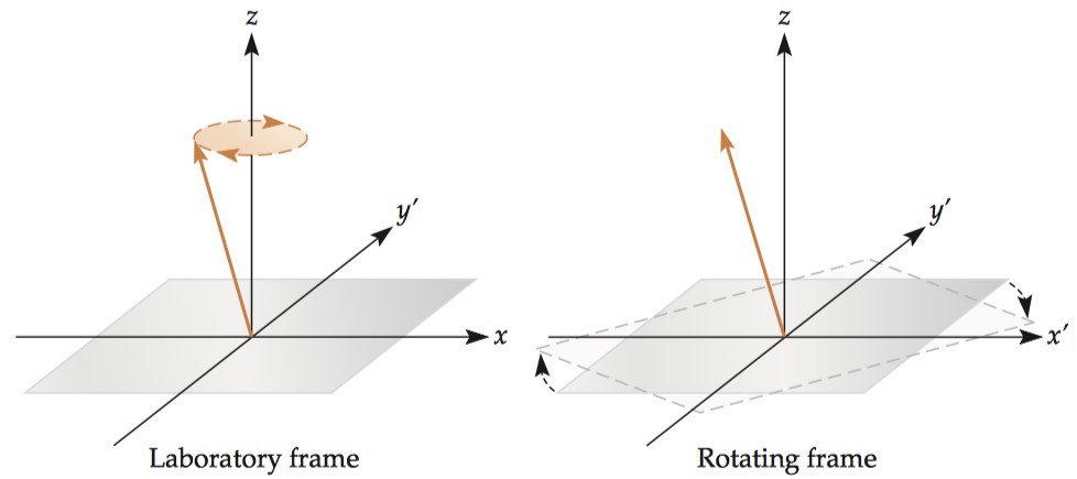 The unit vectors in the transverse plane within the rotating frame are represented by \(\vec{x^′}\) and \(\vec{y^′}\) and correspond to the following unit vectors in the laboratory frame.
\[
\left \{
\begin{array}{l}
\vec{x'}=\vec{x}\cos ωt-\vec{y}\sin ωt \\
\vec{y'}=\vec{x}\sin ωt+\vec{y}\cos ωt
\end{array}
\right.
\]
Within the rotating frame, both the spins and the excitation pulse become stationary, making subsequent formulas much simpler.
\[\vec M= M_0 \vec z\]
\[\vec B_1 = B_1 \vec{x^′}\]
Similarly to single magnetic moment, applying a torque to the net magnetization will rotate its direction over time.
\[\frac{\mathrm{d}\vec{M}}{\mathrm{d}t}=\gamma(\vec{M} \times \vec{B})\]
The torque on the net magnetization depends on the total magnetic field \(\vec{B}\) experienced by the spin system, which is the sum of \(\vec{B_0}\) and \(\vec{B_1}\). If the pulse is presented at the resonant frequency of the sample, called on-resonance excitation, it will rotate the net magnetization vector from the z direction toward the transverse plane. If the pulse is presented at a slightly different frequency, called off-resonance excitation, its efficiency greatly decreases. We define the changing magnetization in the rotating frame as \(\frac{\delta \vec{M}}{\delta t}\) (in contrast to the changing magnetization in the laboratory frame \(\frac{\mathrm{d}\vec{M}}{\mathrm{d}t}\)).
\[
\begin{aligned}
\frac{\mathrm{d}\vec{M}}{\mathrm{d}t}
&=\frac{\mathrm{d}(\vec{x'}M_{x'}+\vec{y'}M_{y'}+\vec{z'}M_{z'})}{\mathrm{d}t}\\
&=(M_{x'}\frac{\mathrm{d}\vec{x'}}{\mathrm{d}t}+M_{y'}\frac{\mathrm{d}\vec{y'}}{\mathrm{d}t})+(\vec{x'}\frac{\mathrm{d}M_{x'}}{\mathrm{d}t}+\vec{y'}\frac{\mathrm{d}M_{y'}}{\mathrm{d}t}+\vec{z'}\frac{\mathrm{d}M_{z'}}{\mathrm{d}t})\\
&=[M_{x'}\frac{\mathrm{d}{(\vec{x}\cos ωt-\vec{y}\sin ωt)}}{\mathrm{d}t}+M_{y'}\frac{\mathrm{d}(\vec{x}\sin ωt+\vec{y}\cos ωt)}{\mathrm{d}t}]+\frac{\delta \vec{M}}{\delta t}\\
&=[M_{x'}\omega(-\vec{y'})+M_{y'}\omega(\vec{x'})]+\frac{\delta \vec{M}}{\delta t}\\
&=-\omega\vec{z}\times \vec M+\frac{\delta \vec{M}}{\delta t}
\end{aligned}
\]
Within the rotating frame, the change in the net magnetization over time, notated as \(\frac{\delta M}{\delta t}\), is determined by the quantity \(B_{1\mathrm{eff}}\), not by \(B_1\) alone.
\[\frac{\delta \vec{M}}{\delta t}=\frac{\mathrm{d}\vec{M}}{\mathrm{d}t}+\omega\vec{z}\times \vec M=\gamma(\vec{M}\times\vec{B})+\omega\vec{z}\times \vec M=\gamma\vec{M}\times(\vec{B}-\frac{\omega\vec{z}}{\gamma})\]
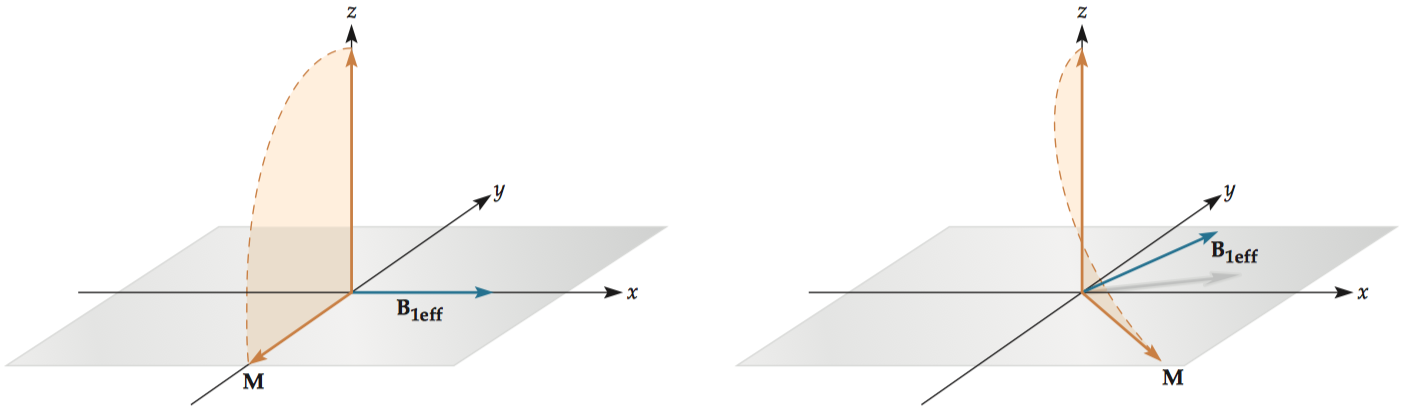
\[\therefore \vec{B_{1\mathrm{eff}}}=\vec{B}-\frac{\omega\vec{z}}{\gamma}=\vec{z}(B_0-\frac{\omega}{\gamma})+\vec{x'}B_1\]
If the excitation pulse (B1 ) is at the resonant frequency of the spin system, so that the term \((B_0-\frac{\omega}{\gamma})\) will be equal to zero. In other words, if the excitation pulse is on-resonance, the net magnetization vector (in the rotating frame) will simply rotate around the x′ component with an angular velocity \(ω_{rot}\).
\[ω_{rot}=\gamma B_{1\mathrm{eff}}=\gamma B_1\]
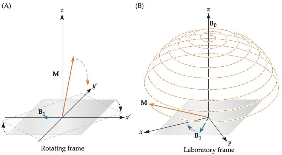
Note that this equation nicely illustrates why g is known as the gyromagnetic ratio, in that it determines the rate at which an introduced magnetic field, in this case \(B_1\), causes a gyroscopic rotation of the net magnetization. In the rotating frame of reference (A), it would look like a simple rotation downward. In the laboratory frame of reference (B), however, the longitudinal magnetization would trace out a complex wobbling path as it rotates downward to the transverse plane. This wobbling motion is known as nutation.
The unit vectors in the transverse plane within the rotating frame are represented by \(\vec{x^′}\) and \(\vec{y^′}\) and correspond to the following unit vectors in the laboratory frame.
\[
\left \{
\begin{array}{l}
\vec{x'}=\vec{x}\cos ωt-\vec{y}\sin ωt \\
\vec{y'}=\vec{x}\sin ωt+\vec{y}\cos ωt
\end{array}
\right.
\]
Within the rotating frame, both the spins and the excitation pulse become stationary, making subsequent formulas much simpler.
\[\vec M= M_0 \vec z\]
\[\vec B_1 = B_1 \vec{x^′}\]
Similarly to single magnetic moment, applying a torque to the net magnetization will rotate its direction over time.
\[\frac{\mathrm{d}\vec{M}}{\mathrm{d}t}=\gamma(\vec{M} \times \vec{B})\]
The torque on the net magnetization depends on the total magnetic field \(\vec{B}\) experienced by the spin system, which is the sum of \(\vec{B_0}\) and \(\vec{B_1}\). If the pulse is presented at the resonant frequency of the sample, called on-resonance excitation, it will rotate the net magnetization vector from the z direction toward the transverse plane. If the pulse is presented at a slightly different frequency, called off-resonance excitation, its efficiency greatly decreases. We define the changing magnetization in the rotating frame as \(\frac{\delta \vec{M}}{\delta t}\) (in contrast to the changing magnetization in the laboratory frame \(\frac{\mathrm{d}\vec{M}}{\mathrm{d}t}\)).
\[
\begin{aligned}
\frac{\mathrm{d}\vec{M}}{\mathrm{d}t}
&=\frac{\mathrm{d}(\vec{x'}M_{x'}+\vec{y'}M_{y'}+\vec{z'}M_{z'})}{\mathrm{d}t}\\
&=(M_{x'}\frac{\mathrm{d}\vec{x'}}{\mathrm{d}t}+M_{y'}\frac{\mathrm{d}\vec{y'}}{\mathrm{d}t})+(\vec{x'}\frac{\mathrm{d}M_{x'}}{\mathrm{d}t}+\vec{y'}\frac{\mathrm{d}M_{y'}}{\mathrm{d}t}+\vec{z'}\frac{\mathrm{d}M_{z'}}{\mathrm{d}t})\\
&=[M_{x'}\frac{\mathrm{d}{(\vec{x}\cos ωt-\vec{y}\sin ωt)}}{\mathrm{d}t}+M_{y'}\frac{\mathrm{d}(\vec{x}\sin ωt+\vec{y}\cos ωt)}{\mathrm{d}t}]+\frac{\delta \vec{M}}{\delta t}\\
&=[M_{x'}\omega(-\vec{y'})+M_{y'}\omega(\vec{x'})]+\frac{\delta \vec{M}}{\delta t}\\
&=-\omega\vec{z}\times \vec M+\frac{\delta \vec{M}}{\delta t}
\end{aligned}
\]
Within the rotating frame, the change in the net magnetization over time, notated as \(\frac{\delta M}{\delta t}\), is determined by the quantity \(B_{1\mathrm{eff}}\), not by \(B_1\) alone.
\[\frac{\delta \vec{M}}{\delta t}=\frac{\mathrm{d}\vec{M}}{\mathrm{d}t}+\omega\vec{z}\times \vec M=\gamma(\vec{M}\times\vec{B})+\omega\vec{z}\times \vec M=\gamma\vec{M}\times(\vec{B}-\frac{\omega\vec{z}}{\gamma})\]
\[\therefore \vec{B_{1\mathrm{eff}}}=\vec{B}-\frac{\omega\vec{z}}{\gamma}=\vec{z}(B_0-\frac{\omega}{\gamma})+\vec{x'}B_1\]
If the excitation pulse (B1 ) is at the resonant frequency of the spin system, so that the term \((B_0-\frac{\omega}{\gamma})\) will be equal to zero. In other words, if the excitation pulse is on-resonance, the net magnetization vector (in the rotating frame) will simply rotate around the x′ component with an angular velocity \(ω_{rot}\).
\[ω_{rot}=\gamma B_{1\mathrm{eff}}=\gamma B_1\]
Note that this equation nicely illustrates why g is known as the gyromagnetic ratio, in that it determines the rate at which an introduced magnetic field, in this case \(B_1\), causes a gyroscopic rotation of the net magnetization. In the rotating frame of reference (A), it would look like a simple rotation downward. In the laboratory frame of reference (B), however, the longitudinal magnetization would trace out a complex wobbling path as it rotates downward to the transverse plane. This wobbling motion is known as nutation.
The flip angle \(\theta\) around which the net magnetization rotates following excitation is determined by the duration T of the applied electromagnetic pulse.
\[\theta=\gamma B_1 T\]
An excitation pulse along the same direction as \(B_0\) would have absolutely no effect, but full excitation can be reached using a slightly off-resonance pulse at the cost of additional time (required to traverse the longer path to the transverse plane).
1.6.2 Signal reception
Change of flux induces an electromotive force (emf) in the coil. By definition, its magnitude is given by \[\mathrm{emf}=-\frac{\mathrm{d}\Phi}{\mathrm{d}t}\] where the magnetic flux penetrating the coil area is given by \[Φ =\int_S B\cdot \mathrm{d}S\] The volume magnetic flux generated by the sample and penetrating through the receiver coil can be represented as \[\Phi(t)=\int_S \bar{B_1}\cdot M(t)\mathrm{d}v \] where \(\bar{B_1}\) is the magnetic field per unit current of the receiver coil and M(t) is the magnetization created by the sample.
If a radiofrequency coil can generate a homogeneous magnetic field within a sample, it can also receive signals uniformly from the sample. This relationship is known as the principle of reciprocity.The additional scaling factor \(\omega_0\) comes from taking the time derivative of M(t), which contains the term \(\omega_0t\). \[\mathrm{emf}=-i\omega_0\int_{v} \bar{B_1}\cdot M(t)\mathrm{d}v\] The amount of MR signal received by the detector coil increases with the square of the magnetic field strength. Unfortunately, the amplitude of noise in the MR signal is proportional to the strength of the magnetic field, so the signal-to-noise ratio increases only linearly with \(B_0\).
1.7 Relaxation Mechanisms of a Spin System
When the excitation pulse is taken away, the spin system gradually loses energy absorbed during the excitation so that spins in the high-energy (antiparallel) state go back to their original state. This phenomenon is known as longitudinal relaxation, or spin–lattice relaxation, because the individual spins lose energy to the surrounding environment, or lattice of nuclei.
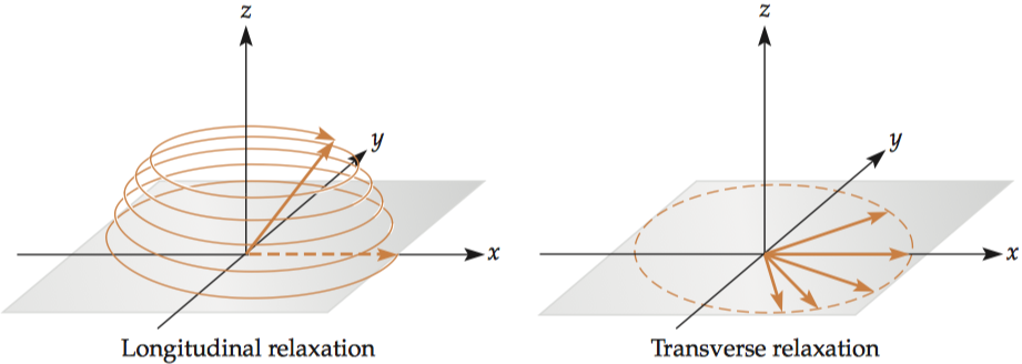
Because the total magnetization is constant, the growth in the longitudinal magnetization corresponds with a reduction in transverse magnetization and a smaller MR signal. The time constant associated with this longitudinal relaxation process is called \(\textbf T_1\), and the relaxation process is called \(\textbf T_1\) recovery. The longitudinal magnetization, \(M_z\), present at time t following an excitation pulse is \[M_z=M_0(1-e^{-\frac{t}{T_1}})\] where \(M_0\) is the original magnetization.
Decay in transverse magnetization \(M_{xy}\) is known as transverse relaxation, or spin–spin relaxation. In general, there are two causes for transverse relaxation(spin–spin interaction), one intrinsic and the other extrinsic (local magnetic field inhomogeneities). \[M_{xy}=M_0e^{-\frac{t}{T_2}}\] The equation for \(T_2^*\) decay is similar to that for \(T_2\) decay.
1.8 The Bloch Equation for MR Signal Generation
Because these components are related, we can describe MR phenomena in a single equation, the Bloch quation, which provides the theoretical foundation for all MRI experiments. \[\frac{\mathrm{d}\vec{M}}{\mathrm{d}t}=\gamma\vec{M} \times \vec{B}+\frac{1}{T_1}(\vec M_0-\vec M_z)-\frac{1}{T_2}(\vec M_x+\vec M_y)\]
2 Basic Principles of MR Image Formation
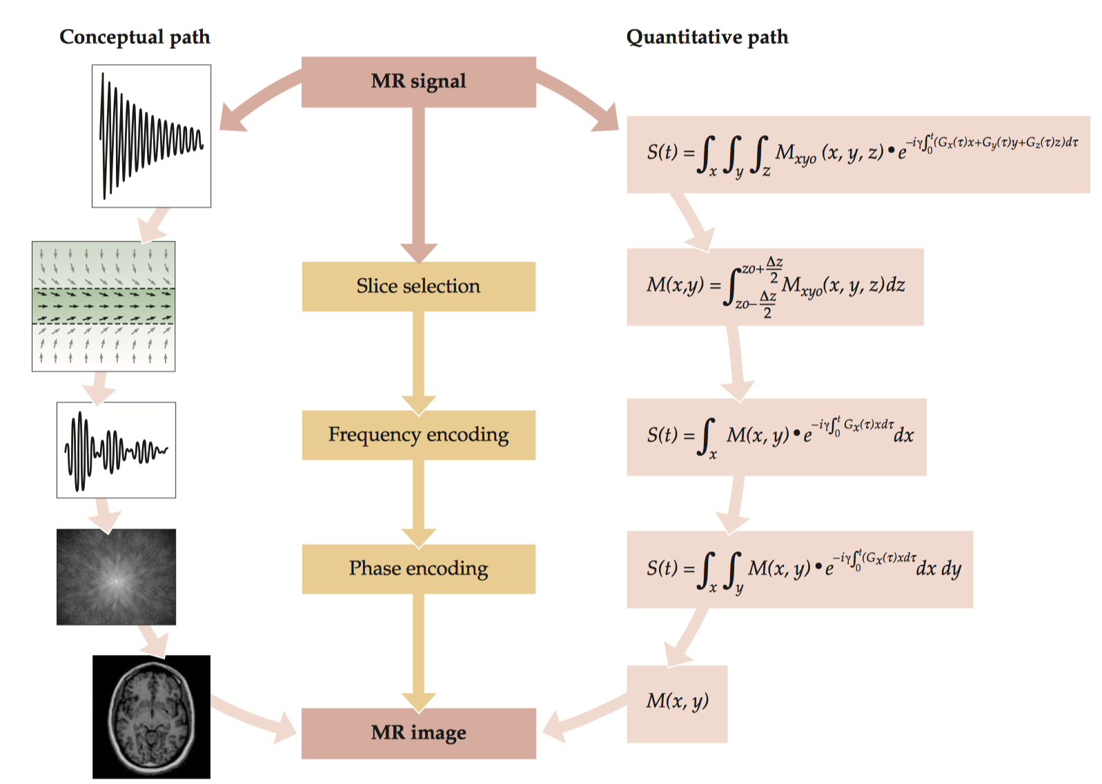
2.1 Conceptual Path
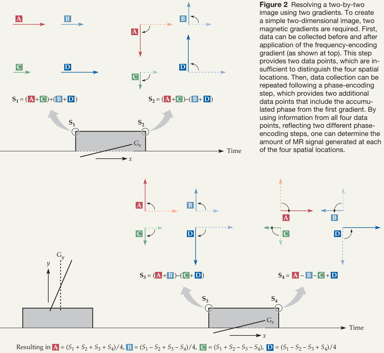
The central innovation that made MR imaging possible was the introduction of superimposed gradient (spatially varying) magnetic fields. To resolve spatial information in three dimensions, we need at least three gradient fields. The gradient magnetic fields along the x, y, and z directions indicate how the strength of that static magnetic field changes in each of the three directions.
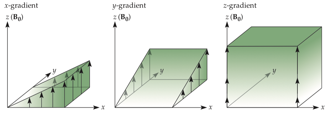
It is critical to remember that the direction of the magnetic field is always along the longitudinal axis; gradient fields change the strength of the static magnetic field at a given spatial location, but not its direction.
The formation of a three-dimensional MR image requires several steps: first, the selection of a slice in which spins will be excited at a particular resonant frequency; then the pre-application of one spatial gradient during phase encoding; and last the application of another gradient for frequency encoding during acquisition of the MR signal.